Random Forest
Imagine you are participating in an important knowledge competition. Facing a difficult problem, would you trust the judgment of one top expert, or the result of a vote by 100 competent contestants? In most cases, collective wisdom can compensate for individual biases and limitations, leading to more stable and accurate decisions.
In the world of machine learning,Random Forestis exactly thiscollective wisdoman outstanding representative of this idea. By building a large number of decision trees and having them vote together to make predictions, it has become one of the most powerful and popular machine learning algorithms.
What is Random Forest?
Random Forestis a machine learning algorithm based on ensemble learning. Its core idea is very simple:Two heads are better than one.。
- Forest: refers to multipledecision trees (Decision Tree)forming a set.
- Random: refers to the two types of randomness introduced by the algorithm when building each decision tree, ensuring that every tree is unique.
Finally, for classification tasks, the forest usesvoting (majority decision)to give results; for regression tasks, it usesaveragingto give results.
Core Idea: Bagging and Randomness
The success of Random Forest rests on two cornerstones:
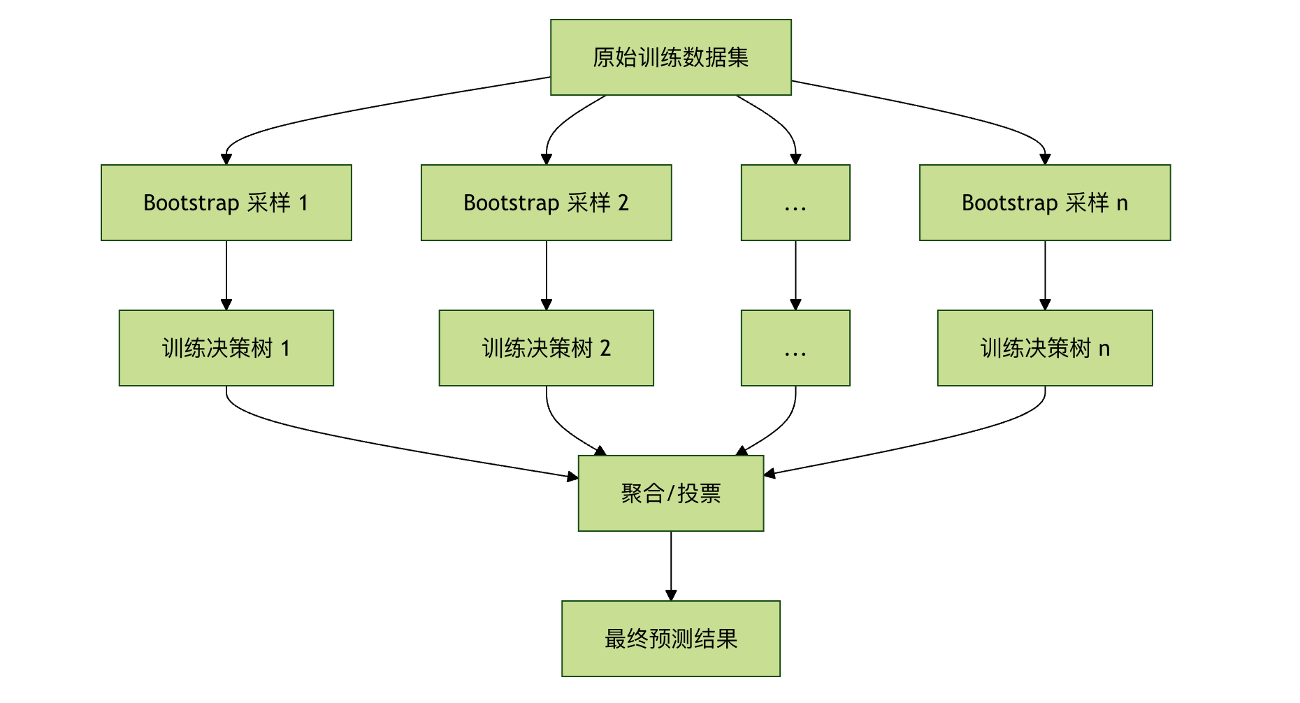
Bagging(Bootstrap Aggregating):
- Bootstrap (Bootstrap Sampling): From the original training dataset,with replacement,randomly draw samples to generate multiple different training subsets. This means the same sample may appear multiple times in one subset, while another sample may not appear at all.
- Aggregating: Use each subset to independently train a decision tree, and finally aggregate the results of all trees (voting or averaging).
Feature Randomness:
- When splitting each node of every tree, the algorithm does not consider all features, but insteadrandomly selects a subset from all features, and then selects the optimal split feature from this subset.
- This further enhances the diversity among trees, allowing the forest to see different aspects of the problem.
In simple terms, Random Forest creates a diversecommittee of experts。Even if some of the trees make mistakes, the other correct trees can correct them through voting, thus achieving more stable and powerful performance than a single decision tree.
Algorithm Workflow and Key Parameters
How Random Forest Works
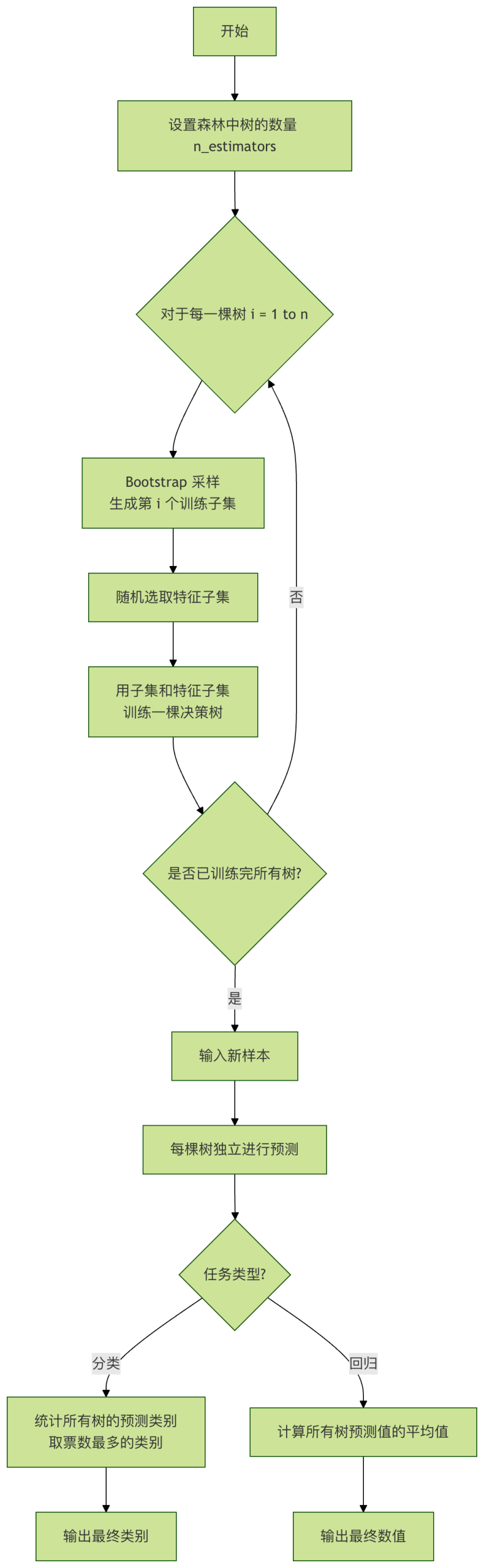
Let's clearly see its working process through a flowchart:
Detailed Explanation of Key Hyperparameters
When using thescikit-learnlibrary, it is crucial to understand the following core parameters:
| Parameter Name | Meaning | Typical Value / Impact | Plain Explanation |
|---|---|---|---|
n_estimators |
The number of decision trees in the forest. | Default is 100. The larger the value, the more stable the model generally is and the better the performance, but the higher the computational cost. | "The number of committee members". The more people, the more reliable the decision is usually, but the longer the meeting takes. |
max_depth |
The maximum depth of a single decision tree. | DefaultNone(no limit). Limiting the depth can prevent overfitting and make the model simpler. |
"Limit each person's speaking time". Prevents an expert (tree) from overthinking and paying excessive attention to details of the training data. |
max_features |
The number of features to consider when searching for the best split. | Can be an integer, a float, or'auto'/'sqrt'. This is the key parameter that introduces "feature randomness". |
"Randomly look at only a few aspects in each discussion". Ensures each tree analyzes the problem from different angles, increasing diversity. |
min_samples_split |
The minimum number of samples required for a node split. | Default is 2. The larger the value, the more conservative the tree growth, and the less likely it is to overfit. | "A group must have at least a few people to continue group discussion". Avoids creating a new rule because of one or two samples. |
min_samples_leaf |
The minimum number of samples required for a leaf node. | Default is 1. The larger the value, the smoother the model. | "The final conclusion should be based on at least a few cases". Ensures every conclusion has sufficient data support. |
bootstrap |
Whether to use Bootstrap sampling. | DefaultTrue. If set toFalse, then the entire dataset will be used to train each tree, but some randomness will be lost. |
"Whether to allow one person to speak repeatedly". Turning it on is the essence of Bagging. |
Hands-on Practice - Code Examples
Let's put it into practice with the classic Iris classification dataset.
Example 1: Basic Classification Task
Example
from sklearn.datasets import load_iris
from sklearn.model_selection import train_test_split
from sklearn.ensemble import RandomForestClassifier
from sklearn.metrics import accuracy_score, classification_report
# 1. Load data
iris = load_iris()
X = iris.data # Features: sepal length, sepal width, petal length, petal width
y = iris.target # Labels: three iris species
# 2. Split training and test sets
X_train, X_test, y_train, y_test = train_test_split(X, y, test_size=0.3, random_state=42)
# 3. Create a Random Forest classifier
# Here we set 100 trees and limit the maximum depth to 5
rf_clf = RandomForestClassifier(n_estimators=100, max_depth=5, random_state=42)
# 4. Train the model
rf_clf.fit(X_train, y_train)
# 5. Make predictions on the test set
y_pred = rf_clf.predict(X_test)
# 6. Evaluate model performance
print("Test set accuracy:", accuracy_score(y_test, y_pred))
print("\nClassification report:")
print(classification_report(y_test, y_pred, target_names=iris.target_names))
Code Explanation:
- Import libraries:
RandomForestClassifieris the Random Forest classifier. - Load data: The Iris dataset has 150 samples, 4 features, and 3 classes.
- Data splitting: Use 70% of the data for training and 30% for testing to validate the model's generalization to new data.
- Instantiate the model:
random_state=42Ensure reproducible results on each run. - Train the model:
fitThe method will build 100 decision trees. - Prediction and evaluation: Use the trained forest to predict on the test set and calculate metrics such as accuracy.
Output:
      setosa       1.00      1.00      1.00        19
  versicolor       1.00      1.00      1.00        13
   virginica       1.00      1.00      1.00        13

    accuracy                           1.00        45
   macro avg       1.00      1.00      1.00        45
weighted avg       1.00      1.00      1.00        45
Example 2: Viewing Feature Importance
Random Forest also has a powerful feature: evaluating the contribution of each feature to predictions.
Example
from sklearn.datasets import load_iris
from sklearn.model_selection import train_test_split
from sklearn.ensemble import RandomForestClassifier
from sklearn.metrics import accuracy_score, classification_report
import pandas as pd
import matplotlib.pyplot as plt
# -------------------------- Set Chinese font start --------------------------
plt.rcParams['font.sans-serif'] = [
# Windows priority
'SimHei', 'Microsoft YaHei',
# macOS priority
'PingFang SC', 'Heiti TC',
# Linux priority
'WenQuanYi Micro Hei', 'DejaVu Sans'
]
# Fix the problem of negative signs displaying as squares
plt.rcParams['axes.unicode_minus'] = False
# -------------------------- Set Chinese font end --------------------------
# 1. Load data
iris = load_iris()
X = iris.data # Features: sepal length, sepal width, petal length, petal width
y = iris.target # Labels: three iris species
# 2. Split training and test sets
X_train, X_test, y_train, y_test = train_test_split(X, y, test_size=0.3, random_state=42)
# 3. Create a Random Forest classifier
# Here we set 100 trees and limit the maximum depth to 5
rf_clf = RandomForestClassifier(n_estimators=100, max_depth=5, random_state=42)
# 4. Train the model
rf_clf.fit(X_train, y_train)
# 5. Make predictions on the test set
y_pred = rf_clf.predict(X_test)
# 6. Evaluate model performance
print("Test set accuracy:", accuracy_score(y_test, y_pred))
print("\nClassification report:")
# Get feature importance
feature_importances = rf_clf.feature_importances_
features = iris.feature_names
# Create a DataFrame for easier viewing
importance_df = pd.DataFrame({
'Feature': features,
'Importance': feature_importances
}).sort_values('Importance', ascending=False)
print("Feature importance ranking:")
print(importance_df)
# Visualization
plt.figure(figsize=(8, 5))
plt.barh(importance_df['Feature'], importance_df['Importance'])
plt.xlabel('Feature Importance')
plt.title('Random Forest - Feature Importance')
plt.gca().invert_yaxis() # Make the most important features appear at the top
plt.show()
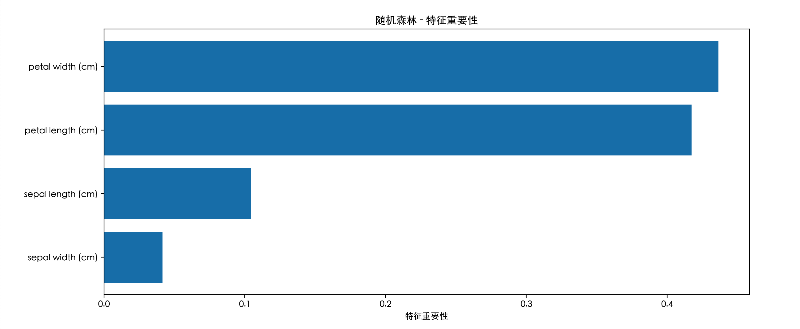
Output analysis:You may find that petal length and petal width are far more important than sepal dimensions. This is highly consistent with botanical common sense; petal features are indeed the key to distinguishing different iris flowers.This feature is extremely valuable for feature selection and data understanding.
Part 4: Advantages, Disadvantages, and Application Scenarios
Advantages
- High accuracy:Ensemble learning can usually achieve top-tier performance on the given data.
- Strong resistance to overfitting:Thanks to Bagging and random feature selection, it is not easy to overfit even without pruning.
- Friendly data requirements:Can handle numerical and categorical features without requiring feature scaling (e.g., normalization).
- Provides feature importance:Built-in feature evaluation is a valuable byproduct.
- Easy to parallelize:The training of each tree is independent and can be easily accelerated in parallel.
Disadvantages
- Poor model interpretability:A "black box" composed of hundreds or thousands of trees is much harder to interpret than a single decision tree.
- Slow training and prediction speed:When the number of trees is large, more computing resources and time are required.
- Large memory footprint:It is necessary to store all tree structures of the entire forest.
Typical Application Scenarios
- Classification problems:Such as spam detection, disease diagnosis, image classification.
- Regression problems:Such as house price prediction, sales forecasting.
- Feature selection:Use the feature importance it outputs for feature filtering.
- Missing value handling:Random forests have a natural ability to handle missing values well.