Machine Learning - PCA Visualization Case
Imagine you are tidying up a cluttered room filled with various items. To better understand the layout of the room, you might take several photos from different angles (e.g., front, side, top-down).
Principal Component Analysis (PCA)does something similar in machine learning.
PCA is a powerfuldata dimensionality reductionandand visualizationtool. When our data contains hundreds or thousands of features (dimensions), the data is like being in an ultra-high-dimensional space that humans cannot intuitively understand.
PCA helps us find the most important perspectives (i.e., principal components) in the data and projects the data onto the most important two or three dimensions, allowing us to observe the structure and distribution of high-dimensional data using two-dimensional or three-dimensional scatter plots.
In simple terms, the goals of PCA are:
- Dimensionality reduction:Use fewer features to represent the original data, reducing computation and storage space while removing noise.
- Visualization:Reduce high-dimensional data to 2D or 3D so that we can intuitively observe the relationships between data points (e.g., clustering, separation).
PCA Core Principles and Workflow
The core idea of PCA is to find the directions in which the data variance is maximized.
The larger the variance, the more dispersed the projected points are in that direction, and the more information they contain.
The first direction found is thefirst principal component (PC1),and the second direction, which is orthogonal to PC1 and has the next largest variance, is thesecond principal component (PC2),and so on.
PCA Workflow Diagram
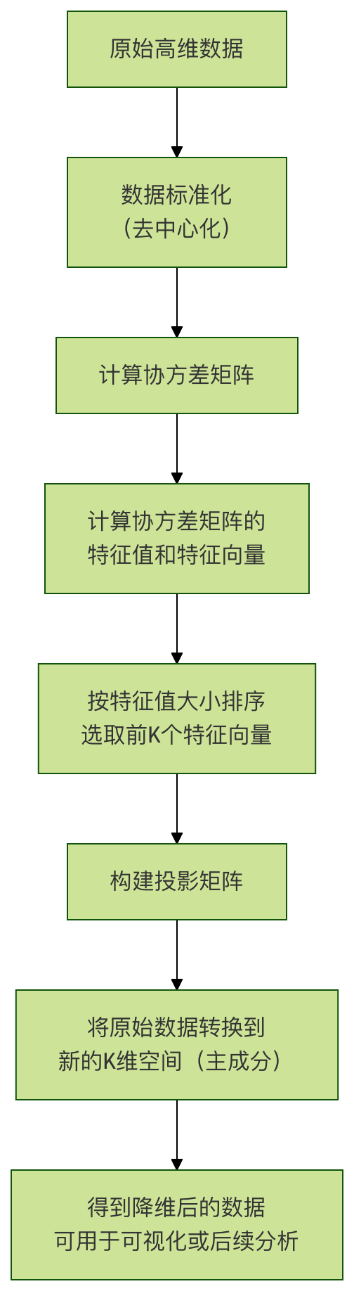
Key steps in the workflow:
Standardization:Make each feature have a mean of 0 and a standard deviation of 1, ensuring all features have equal importance during computation.
Covariance matrix:Calculate the correlations between features. PCA finds the main directions of data variation by analyzing this matrix.
Eigenvalues and Eigenvectors:
- Eigenvectors:These are the principal component directions we are looking for.
- Eigenvalues:They correspond to the data variance along the direction of the eigenvector. The larger the eigenvalue, the more important the corresponding principal component.
Selecting Principal Components:We sort the eigenvalues from largest to smallest and select the eigenvectors corresponding to the top K largest eigenvalues. K is the target dimensionality we want to reduce to (e.g., for visualization, K=2 or 3).
Data Transformation:Use the selected K eigenvectors to form a projection matrix, then multiply the original data by this matrix to obtain the coordinates on the K new principal components, i.e., the reduced data.
Practical Case: Visualization of the Iris Dataset
We will use the classicIris datasetto demonstrate PCA. This dataset contains 150 samples, each with 4 features (sepal length, sepal width, petal length, petal width), and belongs to 3 different species.
Our goal is to use PCA to reduce this 4-dimensional data to 2 dimensions and plot it on a 2D plane to see whether different species of flowers can be distinguished.
Environment Preparation and Data Loading
First, ensure you have installed the necessary Python libraries:scikit-learn, matplotlib, numpy,pandas。
Example
import numpy as np
import pandas as pd
import matplotlib.pyplot as plt
from sklearn import datasets
from sklearn.decomposition import PCA
from sklearn.preprocessing import StandardScaler
# Set Chinese font and chart style (optional)
plt.rcParams['font.sans-serif'] = ['SimHei'] # Used to display Chinese labels properly
plt.rcParams['axes.unicode_minus'] = False # Used to display negative signs properly
# Load the Iris dataset
iris = datasets.load_iris()
X = iris.data # Feature data, shape (150, 4)
y = iris.target # Target labels (species), shape (150,)
target_names = iris.target_names # Species names: ['setosa', 'versicolor', 'virginica']
print(f"Dataset shape: {X.shape}")
print(f"Feature names: {iris.feature_names}")
print(f"Target classes: {target_names}")
Output:
数据集形状: (150, 4)
特征名称: ['sepal length (cm)', 'sepal width (cm)', 'petal length (cm)', 'petal width (cm)']
目标类别: ['setosa' 'versicolor' 'virginica']
Data Standardization
Before applying PCA, standardizing the data is acrucialstep.
Because PCA is very sensitive to the scale of features. If one feature has a numerical range (e.g., petal length measured in centimeters, values between 1-10) much larger than another feature (e.g., sepal width measured in millimeters, values between 0.1-1), then the feature with the larger range will dominate the direction of the principal components, which is usually not what we want.
Example
scaler = StandardScaler()
X_scaled = scaler.fit_transform(X)
print("After standardization, the first 5 samples:")
print(X_scaled[:5])
Applying PCA for Dimensionality Reduction
We use thescikit-learnofPCAPCA class, which can easily complete all the mathematical calculations.
Example
pca = PCA(n_components=2)
# Fit the PCA model on the standardized data and transform the data
X_pca = pca.fit_transform(X_scaled)
print(f"Reduced data shape: {X_pca.shape}")
print(f"Coordinates of the first 5 samples on PC1 and PC2:\n{X_pca[:5]}")
# Check the variance explained ratio of each principal component
print(f"Principal component variance explained ratio: {pca.explained_variance_ratio_}")
print(f"Cumulative variance explained ratio of the first two principal components: {sum(pca.explained_variance_ratio_):.4f}")
Code explanation:
n_components=2: Specifies that we want to reduce the data to 2 dimensions.
fit_transform(X_scaled): This method completes two things at once:
fit: Based on the input data,X_scaledcalculate the parameters required by PCA (such as principal component directions).transform: Use the calculated parameters toX_scaledtransform the data into the new two-dimensional space.
explained_variance_ratio_: This is a very important attribute. It tells us theproportion of the original data variance captured by each principal component.For example, if the output is[0.73, 0.23], it means PC1 retains 73% of the information in the original data, PC2 retains 23%, and together they retain 96% of the information. This helps us evaluate the information loss after dimensionality reduction.
Visualization Results
Now, we have the two-dimensional dataX_pca, and we can easily visualize it with a scatter plot.
Example
plt.figure(figsize=(8, 6))
# Set different colors and markers for each species
colors = ['navy', 'turquoise', 'darkorange']
lw = 2 # Line width
# Loop through the three species and plot each
for color, i, target_name in zip(colors, [0, 1, 2], target_names):
plt.scatter(X_pca[y == i, 0], # Select the PC1 coordinates of samples belonging to species i
X_pca[y == i, 1], # Select the PC2 coordinates of samples belonging to species i
color=color, alpha=0.8, lw=lw,
label=target_name)
# Add chart title and axis labels
plt.title('PCA 2D Visualization of the Iris Dataset')
plt.xlabel(f'First Principal Component (PC1) - Variance explained ratio: {pca.explained_variance_ratio_)
plt.ylabel(f'Second Principal Component (PC2) - Variance explained ratio: {pca.explained_variance_ratio_)
plt.legend(loc='best', shadow=False, scatterpoints=1)
plt.grid(True, linestyle='--', alpha=0.6)
# Display the chart
plt.tight_layout()
plt.show()
Interpretation of the visualization results:After running the above code, you will get a two-dimensional scatter plot.
- X-axis (PC1): Represents the direction of maximum variance among the original 4 features and is the most important dimension for distinguishing data. As can be seen from the figure, it separates theSetosaspecies well from the other two species.
- Y-axis (PC2): Represents the direction orthogonal to PC1 with the second largest variance and provides additional distinguishing information. It helps further distinguishVersicolorandVirginica (Virginia Iris), although the two have some overlap.
- Conclusion: Through PCA, we successfully projected the 4-dimensional data onto a 2D plane and clearly observed the clustering of the three species. Setosa is completely separated, while Versicolor and Virginica partially overlap in the 2D projection, indicating that using only the first two principal components (retaining about 95% of the information) is not enough to perfectly distinguish the latter two species, but their main distribution trends are already very obvious.
Further Exploration and Thinking
How to Choose the Number of Principal Components (K value)?
In real projects, we may not know how many dimensions to reduce to. A common method is to plot aScree Plot, which shows the variance explained rate of each principal component.
Example
pca_full = PCA()
pca_full.fit(X_scaled)
# Plot the scree plot
plt.figure(figsize=(8, 5))
plt.plot(range(1, len(pca_full.explained_variance_ratio_) + 1),
pca_full.explained_variance_ratio_, 'o-', linewidth=2)
plt.title('PCA Variance Explained Rate Scree Plot')
plt.xlabel('Principal Component Index')
plt.ylabel('Variance Explained Rate')
plt.grid(True, linestyle='--', alpha=0.6)
plt.xticks(range(1, len(pca_full.explained_variance_ratio_) + 1))
plt.tight_layout()
plt.show()
# Plot the cumulative variance explained rate
plt.figure(figsize=(8, 5))
plt.plot(range(1, len(pca_full.explained_variance_ratio_) + 1),
np.cumsum(pca_full.explained_variance_ratio_), 's-', linewidth=2, color='red')
plt.title('PCA Cumulative Variance Explained Rate')
plt.xlabel('Number of Principal Components')
plt.ylabel('Cumulative Variance Explained Rate')
plt.axhline(y=0.95, color='gray', linestyle='--', label='95% threshold') # Common threshold
plt.legend()
plt.grid(True, linestyle='--', alpha=0.6)
plt.xticks(range(1, len(pca_full.explained_variance_ratio_) + 1))
plt.tight_layout()
plt.show()
How to choose the K value?
- Look at the elbow point: In the scree plot, find the point where the decrease in variance explained rate suddenly slows down (i.e., the elbow). The principal components after it contribute less.
- Set a threshold: In the cumulative variance plot, choose the smallest K value that makes the cumulative explained rate reach a satisfactory threshold (such as 95% or 99%). From the cumulative plot of the iris data, the first two principal components already explain more than 95% of the variance, so K=2 is a good choice.
Understanding the Meaning of Principal Components
We can also look at the principal components'Loadings, i.e., the contribution weights of each original feature to the principal components, which helps to interpret the actual meaning of the principal components.
Example
pca_components = pca.components_ # Shape is (2, 4)
# Use a DataFrame for clearer display
df_components = pd.DataFrame(pca_components,
columns=iris.feature_names,
index=['PC1', 'PC2'])
print("Principal component loading matrix (eigenvectors):")
print(df_components)
# Can be visualized with a heatmap
import seaborn as sns
plt.figure(figsize=(8, 4))
sns.heatmap(df_components, annot=True, cmap='RdBu_r', center=0)
plt.title('Principal Component Loading Heatmap')
plt.tight_layout()
plt.show()
Interpreting the loading matrix:
- ForPC1, if petal length and petal width have relatively largecorrectweights, while sepal width has relatively largenegativeweights, then PC1 may mainly represent the comprehensive feature of the contrast between petal size and sepal width.
- ForPC2, the weight pattern is different, and it may represent another combination of features. By analyzing these weights, we can assign some practical biological or business meaning to the abstract principal components.
Summary and Practice Exercises
Key Points Summary
- What is PCA: An unsupervised linear dimensionality reduction method that re-expresses data by finding the orthogonal directions (principal components) with maximum data variance.
- Core Steps: Standardization -> Compute covariance matrix -> Compute eigenvalues and eigenvectors -> Select principal components -> Project data.
- Important Concepts:
- Principal Components: New, uncorrelated feature axes.
- Variance Explained Rate: A metric that measures the importance of each principal component.
- Loadings: The bridge connecting original features and principal components, used to explain the meaning of principal components.
- Main Applications: Data visualization, removing noise and redundancy, and serving as a preprocessing step for other models (such as classification, regression) to speed up training.
Hands-on Practice
To consolidate your knowledge, please try to complete the following exercises:
Exercise 1: Explore Different DatasetsTry toscikit-learnin other datasets (such asdigitshandwritten digit dataset orwinewine dataset) to perform PCA visualization. Observe whether the reduced-dimensional images can still retain the discrimination between different categories.
Example
from sklearn.datasets import load_wine
wine = load_wine()
# ... Repeat the PCA process
Exercise 2: 3D VisualizationReduce the iris data to 3 dimensions, and usempl_toolkits.mplot3dlibrary to draw a 3D scatter plot. See whether the overlap between Versicolor and Virginica decreases after adding one dimension.
Example
pca3 = PCA(n_components=3)
X_pca3 = pca3.fit_transform(X_scaled)
# ... Create a 3D figure for plotting