K-Nearest Neighbors Algorithm
K-Nearest Neighbors (KNN) is a simple and commonly used classification and regression algorithm.
K-Nearest Neighbors is a type of supervised learning. Its core idea is to calculate the distance between the sample to be classified and each sample in the training set, find the K samples with the smallest distance, and then predict the class or value of the target sample based on the classes or values of these K samples.
Basic Principles of KNN
The basic principles of the KNN algorithm can be summarized as the following steps:
- Compute Distance: Calculate the distance between the sample to be classified and each sample in the training set. Common distance metrics include Euclidean distance, Manhattan distance, etc.
- Select K Nearest Neighbors: Based on the calculated distances, select the K samples with the smallest distance.
- Voting or Averaging: For classification problems, the class that appears most frequently among the K nearest neighbors is the class of the target sample; for regression problems, the average value of the K nearest neighbors is the value of the target sample.
Features of KNN
- Simple and Easy to Understand: The principle of the KNN algorithm is very simple, easy to understand and implement.
- No Training Required: KNN is a "lazy learning" algorithm that does not require an explicit training process; all computations are performed at prediction time.
- No Assumptions about Data Distribution: KNN does not make any assumptions about the data distribution, making it suitable for various types of data.
- High Computational Complexity: Since KNN needs to calculate distances to all samples at prediction time, the computational complexity becomes high when the dataset is large.
Advantages and Disadvantages of KNN Algorithm
Advantages
- Simple and Easy to Use: The KNN algorithm is simple in principle and easy to understand and implement.
- No Training Required: KNN does not require an explicit training process; all computations are performed at prediction time.
- Suitable for Multi-class Classification: KNN can easily handle multi-class classification problems.
Disadvantages
- High Computational Complexity: KNN needs to calculate distances to all samples at prediction time, and the computational complexity is high when the dataset is large.
- Sensitive to Noise: KNN is relatively sensitive to noisy data, which may affect prediction results.
- Need to Choose an Appropriate K Value: The choice of K value greatly affects model performance, and selecting an appropriate K value is a challenge.
Implementation Steps of KNN Algorithm
1. Import Necessary Libraries
First, we need to import some common Python libraries, such asnumpyfor numerical computation,matplotlibfor plotting,sklearnfor loading datasets and evaluating models.
Example
import matplotlib.pyplot as plt
from sklearn import datasets
from sklearn.model_selection import train_test_split
from sklearn.neighbors import KNeighborsClassifier
from sklearn.metrics import accuracy_score
2. Load Dataset
We usesklearnfromload_irisfunction to load the classic Iris dataset. This dataset contains 150 samples, each with 4 features, and the goal is to classify samples into 3 classes.
Example
iris = datasets.load_iris()
X = iris.data[:, :2] # Take only the first two features for visualization
y = iris.target
3. Data Preprocessing
Before applying the KNN algorithm, it is usually necessary to standardize the data to ensure that each feature contributes equally to distance calculation.
Example
X_train, X_test, y_train, y_test = train_test_split(X, y, test_size=0.3, random_state=42)
4. Train KNN Model
Next, we usesklearnfromKNeighborsClassifierto train the KNN model. Here we choose K=3, i.e., select 3 nearest neighbors.
Example
knn = KNeighborsClassifier(n_neighbors=3)
# Train the model
knn.fit(X_train, y_train)
5. Prediction and Evaluation
Use the trained model to predict on the test set and calculate the accuracy of the model.
Example
y_pred = knn.predict(X_test)
# Calculate accuracy
accuracy = accuracy_score(y_test, y_pred)
print(f"KNN model accuracy: {accuracy:.4f}")
The output is as follows:
KNN模型的准确率: 0.7556
6. Visualize KNN Classification Results
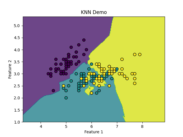
To understand the classification effect of KNN more intuitively, we can plot data points and decision boundaries.
Here we use the first two features of the dataset as input features.
Example
import matplotlib.pyplot as plt
from sklearn import datasets
from sklearn.model_selection import train_test_split
from sklearn.neighbors import KNeighborsClassifier
from sklearn.metrics import accuracy_score
# Load Iris dataset
iris = datasets.load_iris()
X = iris.data[:, :2] # Take only the first two features for visualization
y = iris.target
# Split the dataset into training and test sets
X_train, X_test, y_train, y_test = train_test_split(X, y, test_size=0.3, random_state=42)
# Create KNN model, set K value to 3
knn = KNeighborsClassifier(n_neighbors=3)
# Train the model
knn.fit(X_train, y_train)
# Predict on the test set
y_pred = knn.predict(X_test)
# Calculate accuracy
accuracy = accuracy_score(y_test, y_pred)
print(f"KNN model accuracy: {accuracy:.4f}")
# Plot decision boundary and data points
h = .02 # Mesh step size
x_min, x_max = X[:, 0].min() - 1, X[:, 0].max() + 1
y_min, y_max = X[:, 1].min() - 1, X[:, 1].max() + 1
# Create a 2D mesh grid representing different sample spaces
xx, yy = np.meshgrid(np.arange(x_min, x_max, h),
np.arange(y_min, y_max, h))
# Use the KNN model to predict the class of every point on the grid
Z = knn.predict(np.c_[xx.ravel(), yy.ravel()])
Z = Z.reshape(xx.shape)
# Plot decision boundary
plt.contourf(xx, yy, Z, alpha=0.8)
# Plot training data points
plt.scatter(X[:, 0], X[:, 1], c=y, edgecolors='k', marker='o', s=50)
plt.title("KNN Demo")
plt.xlabel("Feature 1")
plt.ylabel("Feature 2")
plt.show()
The display is as follows:
7. Adjust K Value
The choice of K value has an important impact on model performance.
We usually choose the best K value through cross-validation or visualization methods.
Example
k_range = range(1, 21)
accuracies = []
for k in k_range:
knn = KNeighborsClassifier(n_neighbors=k)
knn.fit(X_train, y_train)
y_pred = knn.predict(X_test)
accuracy = accuracy_score(y_test, y_pred)
accuracies.append(accuracy)
# Plot the relationship between K value and accuracy
plt.plot(k_range, accuracies, marker='o')
plt.title("Relationship between K value and accuracy")
plt.xlabel("K value")
plt.ylabel("Accuracy")
plt.show()
8. Using KNN for Regression Tasks
KNN can also be used for regression tasks (KNN Regression).
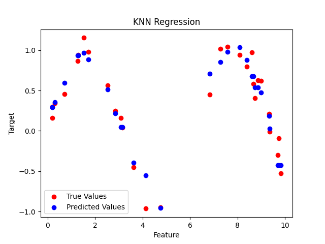
In regression tasks, KNN predicts the output by averaging the target values of the K nearest neighbors.
Example
import matplotlib.pyplot as plt
from sklearn.model_selection import train_test_split
from sklearn.neighbors import KNeighborsRegressor
# Generate sample data
X = np.random.rand(100, 1) * 10
y = np.sin(X).ravel() + 0.1 * np.random.randn(100)
# Split into training and test sets
X_train, X_test, y_train, y_test = train_test_split(X, y, test_size=0.3, random_state=42)
# Create KNN regression model
knn_reg = KNeighborsRegressor(n_neighbors=5)
# Train the model
knn_reg.fit(X_train, y_train)
# Predict on the test set
y_pred = knn_reg.predict(X_test)
# Visualize regression results
plt.scatter(X_test, y_test, color='red', label='True Values')
plt.scatter(X_test, y_pred, color='blue', label='Predicted Values')
plt.title("KNN Regression")
plt.xlabel("Feature")
plt.ylabel("Target")
plt.legend()
plt.show()
Red indicates true values, blue indicates predicted values: