Naive Bayes
Imagine you are browsing an online bookstore, and the system recommends "Ball Lightning" to you based on your previous purchases of "The Three-Body Problem" and "The Wandering Earth". This"Recommended for You"feature likely uses theNaive Bayesalgorithm.
Naive Bayes is aBayes' theorem-based simple and efficientprobabilistic classification algorithm.。
The core idea of Naive Bayes is: through certain known features (such as books you have bought), calculate the probability of an event (such as you liking another book), and select the category with the highest probability as the prediction result.
Its"Naive"lies in a key assumption:all features are mutually independentThat is, when determining whether you like "Ball Lightning", the algorithm considers the two features of having bought "The Three-Body Problem" and having bought "The Wandering Earth" to be unrelated in their influence on your decision. Although in reality features are often correlated, this simplified assumption makes computation very efficient, and works surprisingly well in many practical scenarios (especially text classification).
Core Principle: Bayes' Theorem
To understand Naive Bayes, you must first understand its cornerstone—Bayes' theorem. It describes how to update the probability of an event given certain known conditions.
1. Bayes' Formula
The formula may look a bit abstract, but let's use an example to understand it:
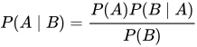
P(A|B) = [P(B|A) * P(A)] / P(B)
Scenario: Determine whether an email is spam (Spam).
- A: The event that the email is "spam".
- B: The feature that the email contains the word "free".
- P(A): The probability that any email is spam, i.e., theprior probability(e.g., based on historical data, 20 out of 100 emails are spam, so P(spam) = 0.2).
- P(B|A): Given that the email is spam, the probability of the word "free" appearing in it, i.e., theconditional probability(e.g., 80% of spam emails contain "free", so P(free|spam) = 0.8).
- P(B): The probability of the word "free" appearing in any email, i.e., theoverall probability。
- P(A|B): What we ultimately want to find: under the conditionthat the email is known to contain the word "free", the probability that this email is spamposterior probability。
The essence of Bayes' theorem: It uses information we already know (the general rule of spamP(A)and spam word usage habitsP(B|A)), combined with newly observed evidence (this email contains "free"), to revise our judgment about this specific event (the likelihood that this email is spamP(A|B))。
2. Where is the "Naive"?
A true Bayesian classifier, when calculatingP(B|A), needs to consider the joint probability of all features (B1, B2, B3...)P(B1, B2, B3... | A), which is very complex.
Naive Bayes makes a powerful simplifying assumption:all features are conditionally independent of each other. This means:
P(B1, B2, B3... | A) ≈ P(B1|A) * P(B2|A) * P(B3|A) * ...
This assumption reduces the complex joint probability calculation to the multiplication of multiple simple probabilities, greatly reducing computational cost.
3. Workflow and Classifier Types
The workflow of a Naive Bayes classifier can be summarized as the following steps:
According to the different types of feature data, Naive Bayes mainly has the following variants:
| Classifier Type | Applicable Feature Data Type | Core Assumption and Description | Typical Application Scenario |
|---|---|---|---|
| Gaussian Naive Bayes | Continuous data | Assumes each feature follows aGaussian distribution (normal distribution)。 | Classify gender based on height and weight; classify iris species based on petal size. |
| Multinomial Naive Bayes | Discrete count data | Assumes features are generated by amultinomial distribution. Particularly suitable fortext classification, where features are usually word occurrence counts or TF-IDF values. | Spam filtering, news topic classification, sentiment analysis (positive/negative reviews). |
| Bernoulli Naive Bayes | Binary data (0/1) | Assumes features arebinary(present or absent), following a Bernoulli distribution. It focuses on "whether it appears", not "how many times it appears". | Text classification (using set-of-words model), user behavior analysis (whether clicked, whether purchased). |
4. Hands-on Practice: Implementing Spam Classification with Python
Let's use a simplified example to implement a spam classifier based on Multinomial Naive Bayes by hand.
1. Scenario and Data Preparation
We have some pre-labeled email texts (spamorhamnormal emails).
Example
train_data = [
("Get the iPhone grand prize for free! Click the link", "spam"),
("Boss, there is a meeting at 3 PM, please attend on time.", "ham"),
("Congratulations, you have won! Claim your prize immediately.", "spam"),
("The project report has been sent to your email, please check.", "ham"),
("Limited-time special price, 50% off on everything, today only", "spam"),
("Weekend dinner is set for 7 PM, the usual place", "ham")
]
2. Code Implementation Steps
Example
from sklearn.feature_extraction.text import CountVectorizer
from sklearn.naive_bayes import MultinomialNB
from sklearn.pipeline import make_pipeline
import numpy as np
# Example training data: each line is an email content followed by a label ('spam' or 'ham')
train_data = [
("Get the iPhone grand prize for free! Click the link", "spam"),
("Boss, there is a meeting at 3 PM, please attend on time.", "ham"),
("Congratulations, you have won! Claim your prize immediately.", "spam"),
("The project report has been sent to your email, please check.", "ham"),
("Limited-time special price, 50% off on everything, today only", "spam"),
("Weekend dinner is set for 7 PM, the usual place", "ham")
]
# 1. Prepare data: separate the text and labels
texts = [data[0] for data in train_data] # Email text list
labels = [data[1] for data in train_data] # Corresponding label list
# 2. Create and train the model pipeline
model = make_pipeline(CountVectorizer(), MultinomialNB())
model.fit(texts, labels)
# 3. Prepare new emails for prediction
new_emails = [
"Get free coupons, a rare opportunity!", # Expected to be spam
"Conference call at 10 a.m. tomorrow to discuss the budget" # Expected to be ham
]
# 4. Make predictions
predictions = model.predict(new_emails)
prediction_proba = model.predict_proba(new_emails) # Get predicted probabilities
# 5. Output results (fix quoting issue + dynamically match probability labels)
# Get the model's category order (avoid hardcoding indices)
class_names = model.classes_
for email, pred, proba in zip(new_emails, predictions, prediction_proba):
# Fix the quote nesting issue: use single quotes for the inner layer, or use single quotes for the outer layer
print(f'Email content: "{email}"')
print(f" Predicted class: {pred}")
# Dynamically output the probability for each class (more robust)
for cls, prob in zip(class_names, proba):
print(f" Probability of belonging to '{cls}': {prob:.4f}")
print("-" * 40)
3. Code Explanation
Data separation: Store the text and labels from the training data into two lists separately; this is thesklearnformat required by the library.
Build the model pipeline:
CountVectorizer(): This is atext feature extractor. It converts each email (a piece of text) into a numeric vector. Each position of the vector represents a word (e.g., "free", "meeting"), and the value represents the number of times that word appears in the email.MultinomialNB(): This is ourMultinomial Naive Bayes classifier. It receives the numeric vectors produced in the previous step, and learns the probabilistic relationship between these vectors and the labels (spam/ham).make_pipeline()It automatically chains these two steps together: transform first, then classify during training, and the same for prediction.
Model training:model.fit(texts, labels)This is the core training process. The algorithm calculates here:
- Prior probability
P(ham)andP(spam)。 - Each word's
hamandspamconditional probability under the categoryP(单词 | ham)andP(单词 | spam)。
Prediction and output: For a new email, the model first converts it into a feature vector, then calculates the probability of it belonging to each category according to the Bayes formula, and finally outputs the category with the higher probability.
Output:
  属于'ham'的概率: 0.5000
  属于'spam'的概率: 0.5000
----------------------------------------
邮件内容: "明天上午十点电话会议讨论预算"
  预测类别: ham
  属于'ham'的概率: 0.5000
  属于'spam'的概率: 0.5000
5. Advantages, Disadvantages, and Cautions
Advantages
- Simple and efficient: The principle is simple, and training and prediction are very fast, making it suitable for large-scale datasets.
- Good performance on small-scale data: Even with limited training data, it can still achieve good results.
- Suitable for high-dimensional data: Especially good at handling data with very high feature dimensions (word count), such as text.
- Relatively robust to irrelevant features: Due to the "naive" independence assumption, individual irrelevant features have little impact on the overall result.
Disadvantages and Cautions
- Limitations of the "naive" assumption: In reality, features are often correlated, and this strong assumption may affect accuracy. For example, in text, "New York" and "Times" often appear together and are not independent.
- Accuracy of probability estimation: The calculated "probability" values are more for classification ranking; their absolute values may not be entirely accurate.
- Zero probability problem: If a feature never appears in a certain category in the training set, its conditional probability is 0, which will cause the entire posterior probability to be 0. The commonly usedLaplace smoothing(in
sklearnvia thealphaparameter setting) is used to solve this, i.e., adding a small constant to the counts of all features to avoid zero values.
6. Exercises and Challenges
To consolidate your understanding of Naive Bayes, try the following exercises:
- Modification exercise: In the above code, try adding more training data, especially emails containing words such as "link", "meeting", and "report", and observe the changes in prediction results and probabilities.
- Parameter tuning: Refer to the
sklearndocumentation to understandMultinomialNB'salphaparameter (smoothing parameter). Try setting it to 0.1, 0.5, 1.0, and see what impact it has on the predicted probabilities. - Changing the classifier: In the code, replace the
MultinomialNB()withBernoulliNB()(Bernoulli Naive Bayes). Note thatCountVectorizermay need to setbinary=Trueto generate binary features. Compare the performance of the two on a simple example. - Practical challenge: Use the
sklearnbuilt-infetch_20newsgroupsdataset (a classic news text classification dataset) and try using Naive Bayes to classify news on different topics.
Naive Bayes is an excellent starting point for learning machine learning. With concise mathematical formulas, it demonstrates the charm of probability theory, and through its practicality, it firmly holds a place in fields such as text classification, recommendation systems, and sentiment analysis. Understanding it means you have grasped the first key to opening the black box of many intelligent applications.
Other extensions