Getting Started with Machine Learning in Python
Python is one of the most commonly used programming languages in machine learning, due to its ease of learning, powerful library support, and community ecosystem.
Next, I will explain step by step how to get started with machine learning using Python, and introduce some common libraries you will need.
Installing Python and necessary libraries
Method 1: Official installer
First, make sure you have installed Python. You can visit the official Python websitehttps://www.python.org/to download and install the latest version.
Windows system:
# 1. 下载安装程序后运行
# 2. 勾选 "Add Python to PATH"
# 3. 选择 "Install for all users"
# 4. 点击 "Install" 开始安装
macOS system:
# 方法1:使用官网安装包
# 下载 .pkg 文件并双击安装
# 方法2:使用 Homebrew
brew install python3
Linux system:
# Ubuntu/Debian
sudo apt update
sudo apt install python3 python3-pip
# CentOS/RHEL
sudo yum install python3 python3-pip
Method 2: Anaconda distribution
Anaconda is a Python distribution designed specifically for data science, just like a "machine learning toolbox" with all tools pre-installed.
Advantages of Anaconda
- Pre-installed common libraries: NumPy, Pandas, Scikit-learn, etc.
- Environment management: conda commands manage virtual environments
- Graphical interface: Anaconda Navigator provides visual operations
- Cross-platform: Supports all major operating systems
Install Anaconda
- Visithttps://www.anaconda.com/products/distribution
- Download the installation package for your system
- Run the installer and follow the prompts to complete the installation
Verify installation:
conda --version
python --version
If you are not yet familiar with Python, you can first study ourPython Tutorial。
If you are not yet familiar with Conda, you can first study ourAnaconda Tutorial。
It is recommended to install Anaconda for creating virtual environments.
Why do you need virtual environments?
A virtual environment is like an independent kitchen prepared for each project, preventing the "seasonings" (library versions) of different projects from interfering with each other.
Benefits of virtual environments
- Dependency isolation: Different projects use different versions of libraries
- Environment reproducibility: Conveniently recreate the same environment on other machines
- Permission management: Avoid polluting the system Python environment
- Project cleanup: Delete the related environment when deleting the project
Managing environments with conda
# 创建环境
conda create -n ml_env python=3.8
# 激活环境
conda activate ml_env
# 安装包
conda install numpy pandas scikit-learn
# 列出环境
conda env list
# 删除环境
conda env remove -n ml_env
Development tool configuration
Jupyter Notebook
Jupyter Notebook is a digital laboratory for data scientists, supporting interactive programming and visual presentation.
Installing and starting Jupyter
# 安装 Jupyter
pip install jupyter
# 启动 Jupyter Notebook
jupyter notebook
# 启动 Jupyter Lab(更现代的界面)
jupyter lab
Basic usage of Jupyter
Example
# Run the following code in Jupyter
# 1. Data import and exploration
import pandas as pd
import numpy as np
import matplotlib.pyplot as plt
# Create sample data
data = {
'Name': ['Zhang San', 'Li Si', 'Wang Wu', 'Zhao Liu'],
'Age': [25, 30, 35, 28],
'City': ['Beijing', 'Shanghai', 'Guangzhou', 'Shenzhen'],
'Salary': [15000, 20000, 18000, 22000]
}
df = pd.DataFrame(data)
print("Data preview:")
print(df.head())
# 2. Data visualization
plt.figure(figsize=(10, 4))
plt.subplot(1, 2, 1)
plt.bar(df['Name'], df['Age'])
plt.title('Age distribution')
plt.xlabel('Name')
plt.ylabel('Age')
plt.subplot(1, 2, 2)
plt.bar(df['Name'], df['Salary'])
plt.title('Salary distribution')
plt.xlabel('Name')
plt.ylabel('Salary')
plt.tight_layout()
plt.show()
# 3. Simple statistical analysis
print("\n"Basic statistical information:")
print(df.describe())
print("\n"City distribution:")
print(df['City'].value_counts())
VS Code configuration
VS Code is a lightweight yet powerful code editor, and through plugins it can become a professional machine learning development environment.
Recommended plugins
- Python: Microsoft official Python plugin
- Jupyter: Supports Jupyter Notebook
- Python Docstring Generator: Automatically generate docstrings
- Bracket Pair Colorizer: Bracket pair colorization
- GitLens: Enhance Git functionality
VS Code configuration example
// .vscode/settings.json
{
    "python.defaultInterpreterPath": "./envs/ml_env/bin/python",
    "python.linting.enabled": true,
    "python.linting.pylintEnabled": true,
    "python.formatting.provider": "black",
    "python.testing.pytestEnabled": true,
    "jupyter.askForKernelRestart": false,
    "editor.fontSize": 14,
    "editor.tabSize": 4,
    "editor.insertSpaces": true
}
Installing machine learning libraries
Common machine learning libraries:
pip install numpy pandas matplotlib seaborn scikit-learn
If you plan to use a deep learning framework, install the following:
pip install torch  # 或者
pip install tensorflow
Related courses:
- Python Tutorial
- Numpy Tutorial
- Pandas Tutorial
- Matplotlib Tutorial
- scikit-learn Tutorial
- PyTorch Tutorial
- OpenCV Tutorial
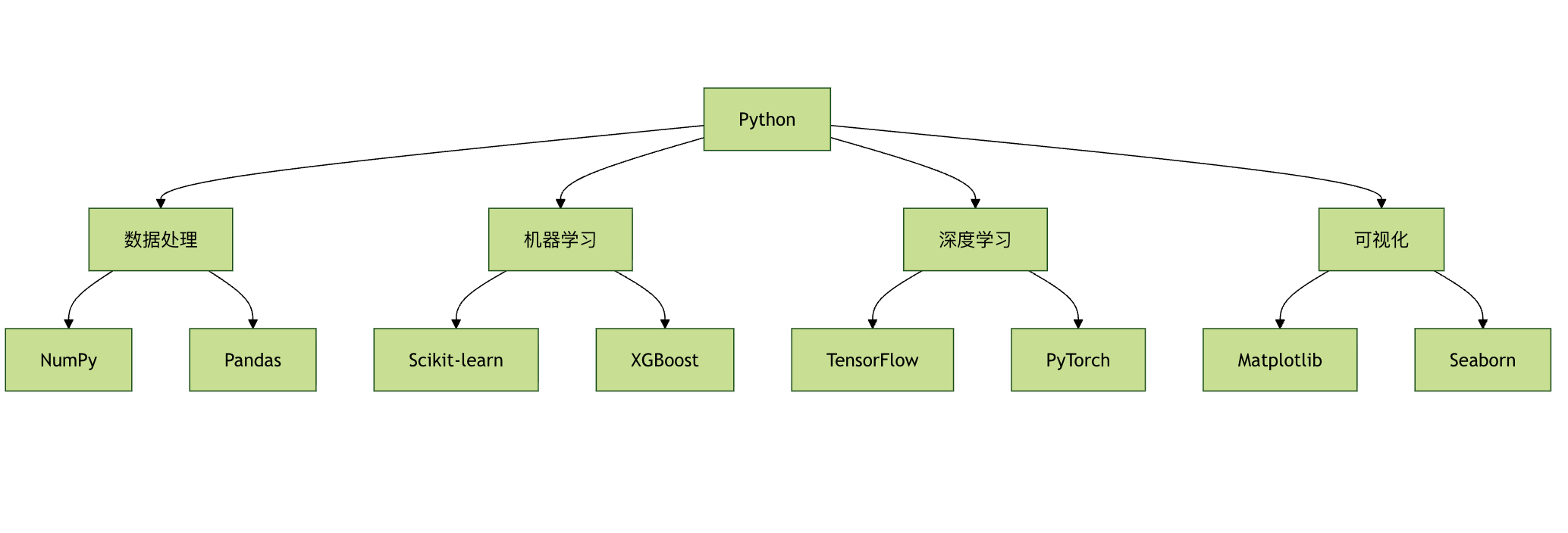
When using Python for machine learning, the entire process generally follows these steps:
Import necessary libraries- For example, NumPy, Pandas, and Scikit-learn.
Load and prepare data- Data is the core of machine learning. You need to load the data and perform necessary preprocessing (e.g., data cleaning, missing value imputation, etc.).
Select models and algorithms- Select suitable machine learning algorithms based on the task (e.g., linear regression, decision trees, etc.).
Train the model- Use the training set data to train the model.
Evaluate the model- Use the test set to evaluate the model's accuracy, and optimize the model based on the evaluation results.
Tune the model and hyperparameters- Adjust the model's hyperparameters based on the evaluation results to further optimize model performance.
A simple machine learning example: classification with Scikit-learn
Scikit-learn (abbreviated as Sklearn) is an open-source machine learning library, built on scientific computing libraries such as NumPy, SciPy, and matplotlib, providing simple and efficient data mining and data analysis tools.
Scikit-learn includes many common machine learning algorithms, including:
- Linear regression, ridge regression, Lasso regression
- Support vector machines (SVM)
- Decision trees, random forests, gradient boosting trees
- Clustering algorithms (e.g., K-Means, hierarchical clustering, DBSCAN)
- Dimensionality reduction techniques (e.g., PCA, t-SNE)
- Neural networks
Next, we will demonstrate the machine learning process using a simple classification task—the Iris Dataset. The Iris dataset is a classic dataset containing 150 samples, describing the petal and sepal lengths and widths of three different types of iris flowers.
Step 1: Import libraries
Import the required Python libraries:
import numpy as np
import pandas as pd
import matplotlib.pyplot as plt
from sklearn.datasets import load_iris
from sklearn.model_selection import train_test_split
from sklearn.preprocessing import StandardScaler
from sklearn.neighbors import KNeighborsClassifier
from sklearn.metrics import accuracy_score
Step 2: Load data
Load the Iris dataset:
Example
iris = load_iris()
# Convert the data to a pandas DataFrame
X = pd.DataFrame(iris.data, columns=iris.feature_names) # Feature data
y = pd.Series(iris.target) # Label data
# Display the first five rows of data
print(X.head())
The printed output data is as follows:
   sepal length (cm)  sepal width (cm)  petal length (cm)  petal width (cm)
0                5.1               3.5                1.4               0.2
1                4.9               3.0                1.4               0.2
2                4.7               3.2                1.3               0.2
3                4.6               3.1                1.5               0.2
4                5.0               3.6                1.4               0.2
Step 3: Split the dataset
Split the dataset into training and test sets, typically using a 70% training set and 30% test set ratio:
Example
X_train, X_test, y_train, y_test = train_test_split(X, y, test_size=0.2, random_state=42)
Step 4: Feature scaling (standardization)
Many machine learning algorithms depend on the scale of features, especially algorithms like K-Nearest Neighbors. To ensure that each feature has a mean of 0 and a standard deviation of 1, we use standardization to process the data:
Example
scaler = StandardScaler()
X_train = scaler.fit_transform(X_train)
X_test = scaler.transform(X_test)
Step 5: Choose a model and train
In this example, we choose the K-Nearest Neighbors (KNN) algorithm for classification:
Example
knn = KNeighborsClassifier(n_neighbors=3)
# Train the model
knn.fit(X_train, y_train)
Step 6: Evaluate the model
After training, we use the test set to evaluate the model's accuracy:
Example
y_pred = knn.predict(X_test)
# Calculate accuracy
accuracy = accuracy_score(y_test, y_pred)
print(f'Model accuracy: {accuracy:.2f}')
After running the above code, the output is:
模型准确率: 1.00
Step 7: Visualize results (optional)
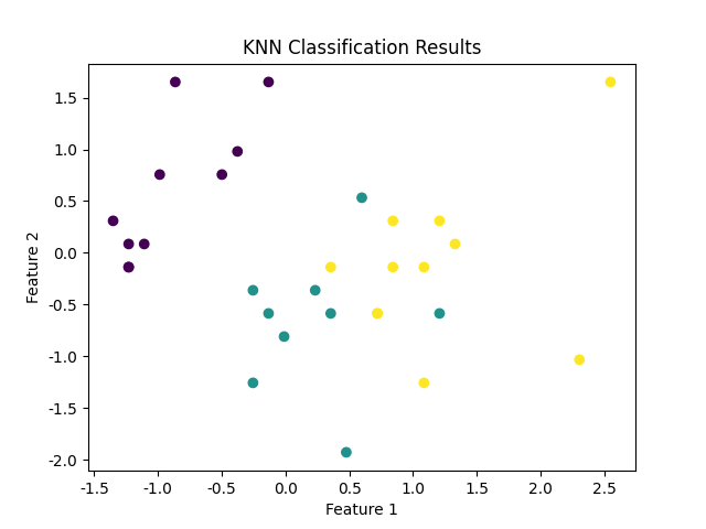
You can further understand the model's performance through visualization, especially with multi-dimensional datasets. For example, you can use a 2D plot to display the KNN classification results (though you need to reduce the dimensionality of the data to two dimensions).
Example
import pandas as pd
import matplotlib.pyplot as plt
from sklearn.datasets import load_iris
from sklearn.model_selection import train_test_split
from sklearn.preprocessing import StandardScaler
from sklearn.neighbors import KNeighborsClassifier
from sklearn.metrics import accuracy_score
# Load the Iris dataset
iris = load_iris()
# Convert data to pandas DataFrame
X = pd.DataFrame(iris.data, columns=iris.feature_names) # Feature data
y = pd.Series(iris.target) # Label data
# Split training and test sets (80% training, 20% test)
X_train, X_test, y_train, y_test = train_test_split(X, y, test_size=0.2, random_state=42)
# Standardize features
scaler = StandardScaler()
X_train = scaler.fit_transform(X_train)
X_test = scaler.transform(X_test)
# Create KNN classifier
knn = KNeighborsClassifier(n_neighbors=3)
# Train the model
knn.fit(X_train, y_train)
# Predict the test set
y_pred = knn.predict(X_test)
# Calculate accuracy
accuracy = accuracy_score(y_test, y_pred)
# Visualization - this is just a simple example; you can choose the plotting method according to the actual situation
plt.scatter(X_test[:, 0], X_test[:, 1], c=y_pred, cmap='viridis', marker='o')
plt.title("KNN Classification Results")
plt.xlabel("Feature 1")
plt.ylabel("Feature 2")
plt.show()
The output image is shown below: