Overfitting, Underfitting, Bias and Variance
In the world of machine learning, building a model is like training a student. Our goal is that thisstudentcan not only memorize the example problems in the textbook (training data), but also deeply understand the underlying principles, so as to achieve good results on completely unseen exam questions (test data). However, thisstudentmay encounter two typical problems during the learning process:
- One is learning too rigidly, merely mechanically applying the examples (underfitting);
- The other is learning too cleverly, memorizing even the punctuation and handwriting characteristics of the examples, so that they are at a loss when facing new questions (overfitting)。
Understandingoverfittingandunderfitting, as well as the deeper theoretical concepts behind them—biasandvariance, is a key step for every machine learning practitioner from beginner to mastery. They explain why models make mistakes and show us the direction for model improvement.
I. Core Concepts: Model Performance and the "Fitting" State
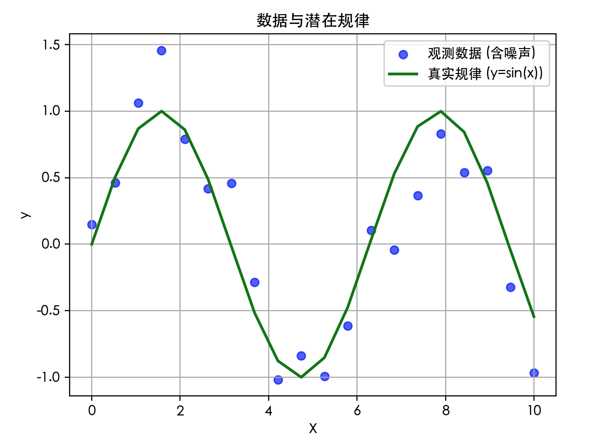
First, let's use an intuitive example to understand whatfittingis. Suppose we want to use a mathematical model to fit a set of scattered data points.
Example
import matplotlib.pyplot as plt
# -------------------------- Set Chinese font start --------------------------
plt.rcParams['font.sans-serif'] = [
# Windows first
'SimHei', 'Microsoft YaHei',
# macOS first
'PingFang SC', 'Heiti TC',
# Linux first
'WenQuanYi Micro Hei', 'DejaVu Sans'
]
# Fix the issue where negative signs display as squares
plt.rcParams['axes.unicode_minus'] = False
# -------------------------- Set Chinese font end --------------------------
# Generate simulated data: add some random noise based on a sine curve
np.random.seed(42)
X = np.linspace(0, 10, 20)
y_true = np.sin(X) # The real underlying pattern (which we don't know)
y_noise = np.random.randn(20) * 0.3 # Random noise
y = y_true + y_noise # The data we actually observe
plt.scatter(X, y, label='Observed data (with noise)', color='blue', alpha=0.6)
plt.plot(X, y_true, label='True pattern (y=sin(x))', color='green', linewidth=2)
plt.xlabel('X')
plt.ylabel('y')
plt.title('Data and underlying pattern')
plt.legend()
plt.grid(True)
plt.show()
Our goal is to find a curve (model) that best describes the pattern reflected by these blue scattered points (data).
The degree to which the model describes the data isfitting。
1. Underfitting
Underfittingrefers to a model that is too simple to capture the basic patterns or structures in the data. It is like a student who has only learned addition but is asked to solve calculus problems.
- Behavior: The model performs very poorly ontraining data(e.g., low accuracy, high error).
- Causes: Model complexity is too low, features are insufficient, or training is inadequate.
- Analogy: Using a straight line (first-degree polynomial) to fit data with an obvious curved trend.
Example
from sklearn.preprocessing import PolynomialFeatures
from sklearn.metrics import mean_squared_error
# Try fitting with a 1st-degree polynomial (straight line)
poly = PolynomialFeatures(degree=1)
X_poly1 = poly.fit_transform(X.reshape(-1, 1))
model_under = LinearRegression()
model_under.fit(X_poly1, y)
y_pred_under = model_under.predict(X_poly1)
mse_train_under = mean_squared_error(y, y_pred_under)
print(f"Underfitting model Mean Squared Error (MSE) on the training set: {mse_train_under:.4f}")
Output:
欠拟合模型在训练集上的均方误差 (MSE): 0.4402
欠拟合模型在训练集上的均方误差 (MSE): 0.4402
2. Just-Right Fit
This is the ideal state. The model is complex enough to learn the key patterns in the data, but not so complex that it learns random noise. It performs well on both the training set and unseen test sets.
- Behavior: The errors on both the training set and the test set are low, and the two are close.
- Analogy: Using a polynomial of appropriate degree (e.g., 3rd degree) to fit the data.
Example
poly = PolynomialFeatures(degree=3)
X_poly3 = poly.fit_transform(X.reshape(-1, 1))
model_good = LinearRegression()
model_good.fit(X_poly3, y)
y_pred_good = model_good.predict(X_poly3)
mse_train_good = mean_squared_error(y, y_pred_good)
print(f"Good-fit model Mean Squared Error (MSE) on the training set: {mse_train_good:.4f}")
Output:
欠拟合模型在训练集上的均方误差 (MSE): 0.4402
良好拟合模型在训练集上的均方误差 (MSE): 0.3988
3. Overfitting
Overfittingrefers to a model that is too complex, learning not only the true patterns in the data but also "memorizing" the random noise and outliers in the training data.
- Behavior: The model performs extremely well ontraining data(with very small error), but onnew, unseen dataits performance drops sharply, showing poor generalization ability.
- Causes: Model complexity is too high, and the amount of training data is too small.
- Analogy: Use a very high-degree polynomial (e.g., 15th degree) to fit the data, causing the curve to pass through almost every data point and become extremely distorted.
Example
import matplotlib.pyplot as plt
from sklearn.linear_model import LinearRegression
from sklearn.preprocessing import PolynomialFeatures
from sklearn.metrics import mean_squared_error
# -------------------------- Set Chinese font start --------------------------
plt.rcParams['font.sans-serif'] = [
# Windows first
'SimHei', 'Microsoft YaHei',
# macOS first
'PingFang SC', 'Heiti TC',
# Linux first
'WenQuanYi Micro Hei', 'DejaVu Sans'
]
# Fix the issue where negative signs display as squares
plt.rcParams['axes.unicode_minus'] = False
# -------------------------- Set Chinese font end --------------------------
# Generate simulated data: add some random noise based on a sine curve
np.random.seed(42)
X = np.linspace(0, 10, 20)
y_true = np.sin(X) # The real underlying pattern (which we don't know)
y_noise = np.random.randn(20) * 0.3 # Random noise
y = y_true + y_noise # The data we actually observe
# Try fitting with a 1st-degree polynomial (straight line)
poly = PolynomialFeatures(degree=1)
X_poly1 = poly.fit_transform(X.reshape(-1, 1))
model_under = LinearRegression()
model_under.fit(X_poly1, y)
y_pred_under = model_under.predict(X_poly1)
mse_train_under = mean_squared_error(y, y_pred_under)
print(f"Underfitting model Mean Squared Error (MSE) on the training set: {mse_train_under:.4f}")
# Try fitting with a 3rd-degree polynomial
poly = PolynomialFeatures(degree=3)
X_poly3 = poly.fit_transform(X.reshape(-1, 1))
model_good = LinearRegression()
model_good.fit(X_poly3, y)
y_pred_good = model_good.predict(X_poly3)
mse_train_good = mean_squared_error(y, y_pred_good)
print(f"Good-fit model Mean Squared Error (MSE) on the training set: {mse_train_good:.4f}")
# Try fitting with a 15th-degree polynomial (extremely prone to overfitting)
poly = PolynomialFeatures(degree=15)
X_poly15 = poly.fit_transform(X.reshape(-1, 1))
model_over = LinearRegression()
model_over.fit(X_poly15, y)
y_pred_over = model_over.predict(X_poly15)
mse_train_over = mean_squared_error(y, y_pred_over)
print(f"Overfitting model Mean Squared Error (MSE) on the training set: {mse_train_over:.4f}")
# Visualize the three fitting states
plt.figure(figsize=(15, 4))
# Underfitting
plt.subplot(1, 3, 1)
plt.scatter(X, y, alpha=0.6)
plt.plot(X, y_pred_under, color='red', linewidth=2, label='Underfitting (1st degree)')
plt.plot(X, y_true, color='green', linestyle='--', label='True pattern')
plt.title(f'Underfitting\nTraining MSE: {mse_train_under:.4f}')
plt.legend()
plt.grid(True)
# Good fit
plt.subplot(1, 3, 2)
plt.scatter(X, y, alpha=0.6)
plt.plot(X, y_pred_good, color='red', linewidth=2, label='Good fit (3rd degree)')
plt.plot(X, y_true, color='green', linestyle='--', label='True pattern')
plt.title(f'Good fit\nTraining MSE: {mse_train_good:.4f}')
plt.legend()
plt.grid(True)
# Overfitting
plt.subplot(1, 3, 3)
plt.scatter(X, y, alpha=0.6)
plt.plot(X, y_pred_over, color='red', linewidth=2, label='Overfitting (15th degree)')
plt.plot(X, y_true, color='green', linestyle='--', label='True pattern')
plt.title(f'Overfitting\nTraining MSE: {mse_train_over:.4f}')
plt.legend()
plt.grid(True)
plt.tight_layout()
plt.show()
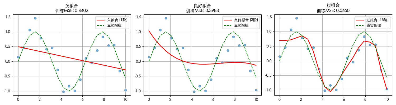
It can be clearly seen from the figure:
- Underfitting (left):The red straight line completely fails to capture the fluctuating trend of the data.
- Good fit (middle):The red curve roughly follows the trend of the green true pattern.
- Overfitting (right):The red curve fluctuates violently, trying to pass through every blue scattered point, including noise points, completely losing the smooth shape of the sine curve.
II. Theoretical Foundations: Bias-Variance Decomposition
Bias and variance provide a theoretical framework for understanding overfitting and underfitting. They describe two different sources of model error.
We can decompose the model'stotal errorinto:Bias² + Variance + Irreducible error。
1. Bias
- Definition: The difference between theexpected value(i.e., the average predicted value) and the true value. It reflects the model's inherentsystematic error, that is, whether the model's assumptions about the nature of the problem are wrong.
- Behavior of high bias: The model is too simple to capture the characteristics of the data, leading tounderfittingNo matter what data is used for training, the results deviate from the true values.
- Example: Always using the simple linear model "house price = area × 1000" to predict all kinds of houses, ignoring important factors such as location and floor level, this is high bias.
2. Variance
- Definition: Thefluctuation rangeof the model's predictions themselves. It reflects the model's sensitivity torandom noisein the training data.
- Symptoms of high variance: The model is too complex and overreacts to small changes (including noise) in the training data, leading tooverfittingTraining on a different set of data may produce a completely different model.
- Example: A deep neural network, if not constrained in any way, may generate a completely different, extremely complex set of prediction rules for each unique training data set, this is high variance.
3. Bias-Variance Tradeoff
This is a core tradeoff in machine learning.We cannot minimize both bias and variance simultaneously.
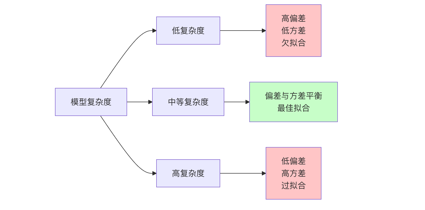
- Increase model complexity: Usually reducesbias(the model becomes more powerful), but increasesvariance(it more easily learns noise).
- Reduce model complexity: Usually reducesvariance(the model becomes more stable), but increasesbias(the model becomes weaker).
Our goal is to find the "sweet spot" in the figure so that the total error is minimized.
III. Diagnosis and Countermeasures
How can we determine which state the model is in? How do we solve it?
1. Diagnostic Method: Learning Curves
A learning curve plots the model's performance (e.g., error) on thetraining setandvalidation setas a function ofthe number of training samplesormodel complexity.
Example
import matplotlib.pyplot as plt
from sklearn.datasets import load_diabetes
from sklearn.model_selection import train_test_split
from sklearn.model_selection import learning_curve
from sklearn.pipeline import make_pipeline
from sklearn.linear_model import LinearRegression
from sklearn.preprocessing import PolynomialFeatures, StandardScaler
from sklearn.metrics import mean_squared_error
import warnings
warnings.filterwarnings('ignore')
# -------------------------- Configure Chinese font start --------------------------
plt.rcParams['font.sans-serif'] = [
# Windows first
'SimHei', 'Microsoft YaHei',
# macOS first
'PingFang SC', 'Heiti TC',
# Linux first
'WenQuanYi Micro Hei', 'DejaVu Sans'
]
# Fix the issue of negative signs displaying as blocks
plt.rcParams['axes.unicode_minus'] = False
# Set chart style
plt.rcParams['figure.figsize'] = (10, 6)
plt.rcParams['axes.grid'] = True
plt.rcParams['grid.alpha'] = 0.3
# -------------------------- Configure Chinese font end --------------------------
# Load data
data = load_diabetes()
X, y = data.data, data.target
# Use only one feature (better for polynomial regression demonstration)
X = X[:, np.newaxis, 2] # Select the third feature (BMI)
X_train, X_test, y_train, y_test = train_test_split(X, y, test_size=0.2, random_state=42)
# Define the learning curve plotting function (optimized version)
def plot_learning_curve(estimator, title, X, y, cv=5, train_sizes=np.linspace(0.1, 1.0, 10)):
"""
Plot the learning curve
Parameters:
estimator: model estimator
title: chart title
X: feature data
y: target variable
cv: number of cross-validation folds
train_sizes: training sample proportions
"""
# Get learning curve data
train_sizes_abs, train_scores, test_scores = learning_curve(
estimator, X, y, cv=cv, scoring='neg_mean_squared_error',
train_sizes=train_sizes, random_state=42, n_jobs=-1
)
# Calculate mean and standard deviation
train_scores_mean = -train_scores.mean(axis=1)
train_scores_std = train_scores.std(axis=1)
test_scores_mean = -test_scores.mean(axis=1)
test_scores_std = test_scores.std(axis=1)
# Plot learning curves
plt.figure(figsize=(10, 6))
plt.fill_between(train_sizes_abs,
train_scores_mean - train_scores_std,
train_scores_mean + train_scores_std,
alpha=0.1, color='r')
plt.fill_between(train_sizes_abs,
test_scores_mean - test_scores_std,
test_scores_mean + test_scores_std,
alpha=0.1, color='g')
# Plot mean curves
plt.plot(train_sizes_abs, train_scores_mean, 'o-', color='r', linewidth=2,
markersize=8, label='Training set MSE')
plt.plot(train_sizes_abs, test_scores_mean, 'o-', color='g', linewidth=2,
markersize=8, label='Validation set MSE')
# Set chart properties
plt.xlabel('Number of training samples', fontsize=12)
plt.ylabel('Mean squared error (MSE)', fontsize=12)
plt.title(title, fontsize=14, pad=20)
plt.legend(loc='upper right', fontsize=11)
plt.tight_layout()
plt.show()
# Print the model's performance on the test set
estimator.fit(X_train, y_train)
y_pred = estimator.predict(X_test)
mse = mean_squared_error(y_test, y_pred)
print(f"{title} - Test set MSE: {mse:.2f}")
# 1. Underfitting model (1st-order polynomial - linear regression)
print("="*60)
print("Underfitting model (1st-order polynomial - linear regression)")
print("="*60)
plot_learning_curve(
make_pipeline(StandardScaler(), PolynomialFeatures(1), LinearRegression()),
'Underfitting model learning curve (1st-order polynomial)',
X, y
)
# 2. Good fitting model (2nd-order polynomial)
print("\n" + "="*60)
print("Good fitting model (2nd-order polynomial)")
print("="*60)
plot_learning_curve(
make_pipeline(StandardScaler(), PolynomialFeatures(2), LinearRegression()),
'Good fitting model learning curve (2nd-order polynomial)',
X, y
)
# 3. Overfitting model (8th-order polynomial)
print("\n" + "="*60)
print("Overfitting model (8th-order polynomial)")
print("="*60)
plot_learning_curve(
make_pipeline(StandardScaler(), PolynomialFeatures(8), LinearRegression()),
'Overfitting model learning curve (8th-order polynomial)',
X, y
)
# Extra: visualize the fitting effects of models with different orders
plt.figure(figsize=(12, 8))
X_plot = np.linspace(X.min(), X.max(), 100).reshape(-1, 1)
# Plot original data points
plt.scatter(X_train, y_train, alpha=0.5, label='Training data', color='blue', s=30)
plt.scatter(X_test, y_test, alpha=0.5, label='Test data', color='orange', s=30)
# Plot fitting curves for different orders
orders = [1, 2, 8]
colors = ['red', 'green', 'purple']
labels = ['1st-order (underfitting)', '2nd-order (good fitting)', '8th-order (overfitting)']
for i, order in enumerate(orders):
model = make_pipeline(StandardScaler(), PolynomialFeatures(order), LinearRegression())
model.fit(X_train, y_train)
y_plot = model.predict(X_plot)
plt.plot(X_plot, y_plot, color=colors[i], linewidth=2, label=labels[i])
plt.xlabel('BMI feature (standardized)', fontsize=12)
plt.ylabel('Diabetes progression index', fontsize=12)
plt.title('Comparison of polynomial regression fitting effects with different orders', fontsize=14, pad=20)
plt.legend(fontsize=11)
plt.tight_layout()
plt.show()
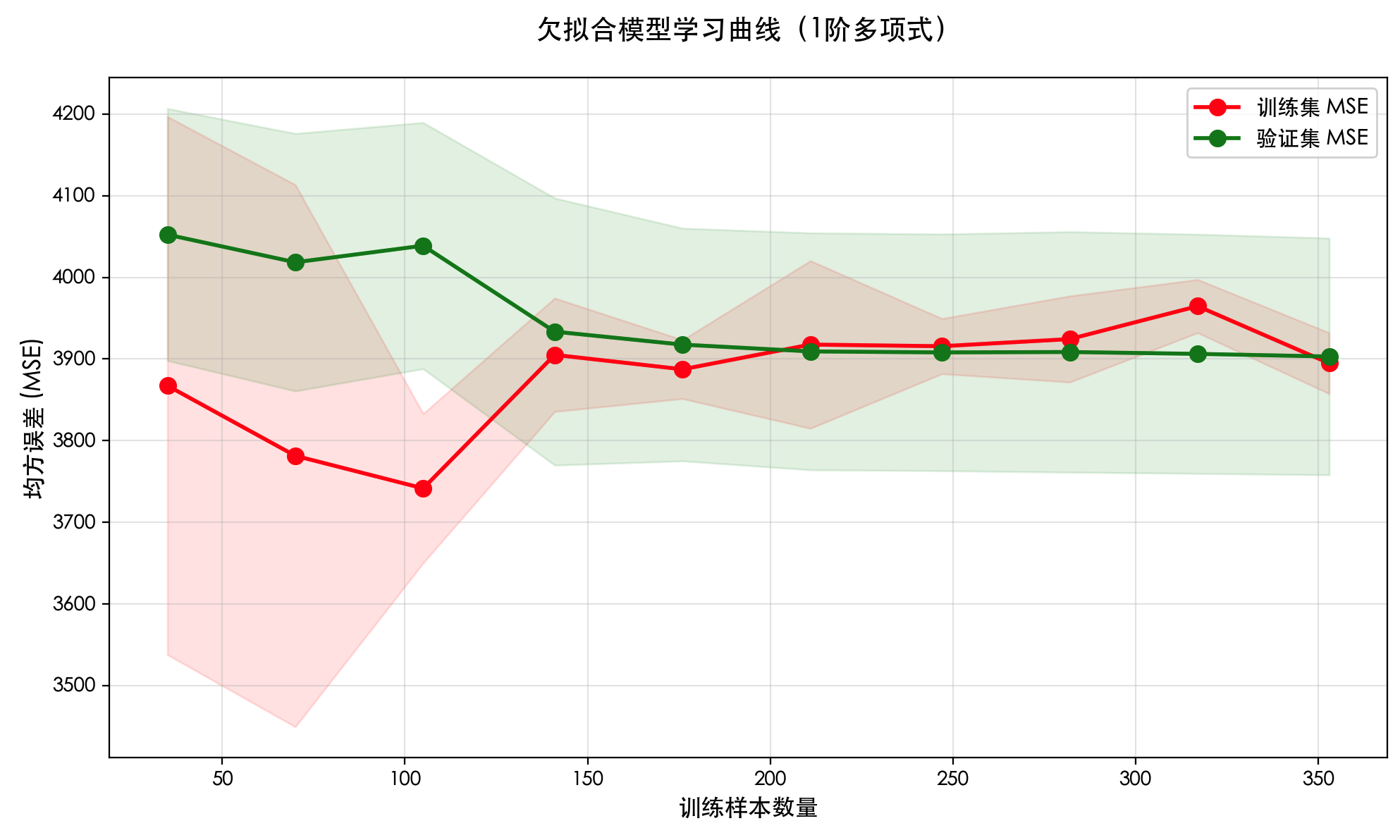
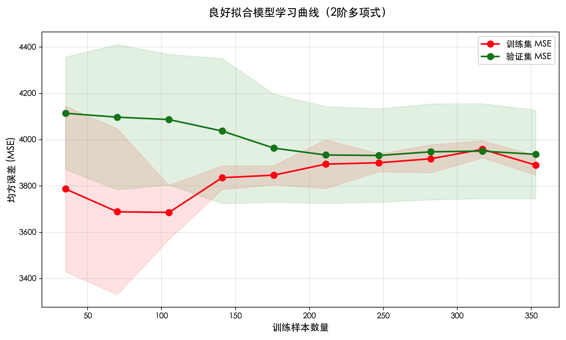
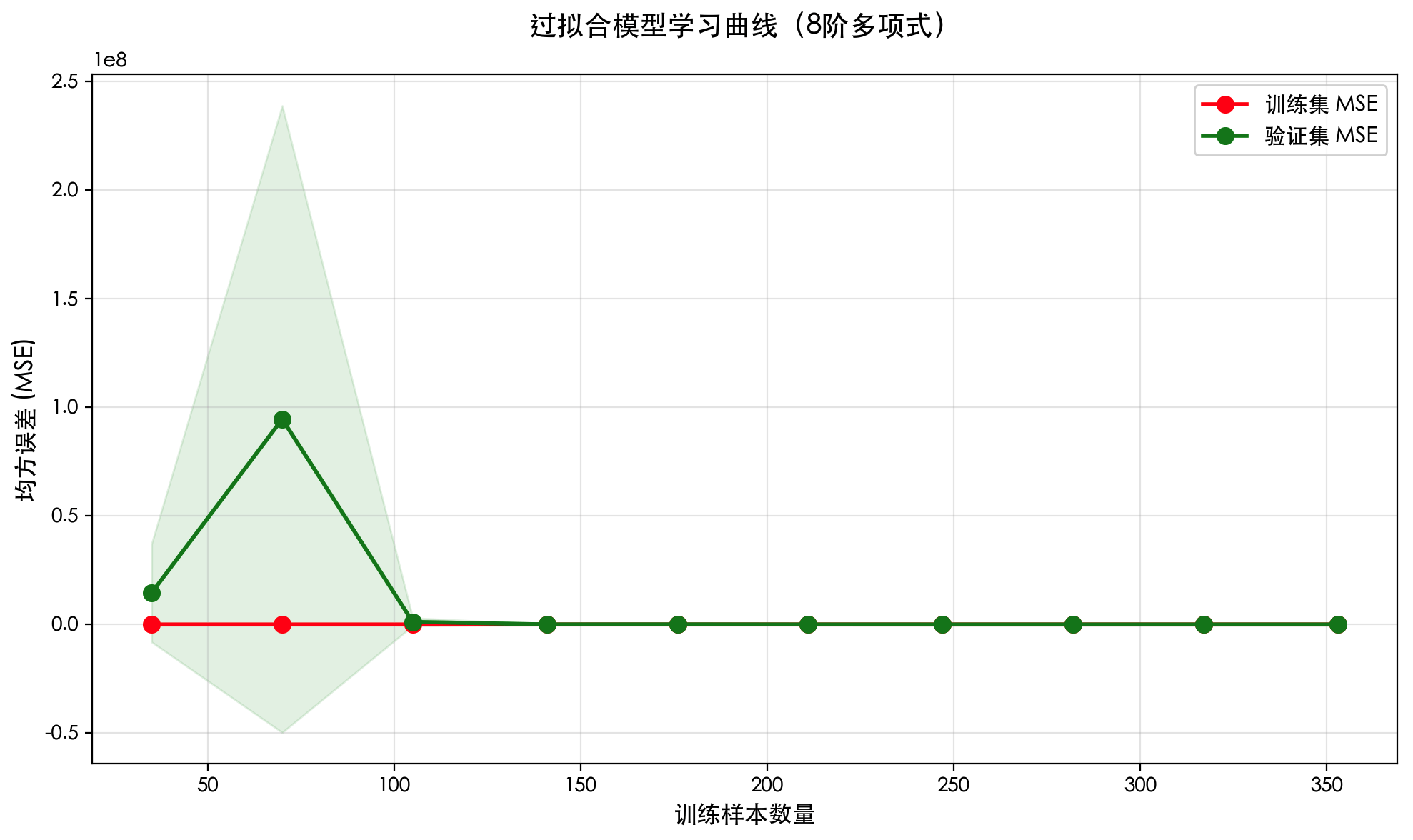
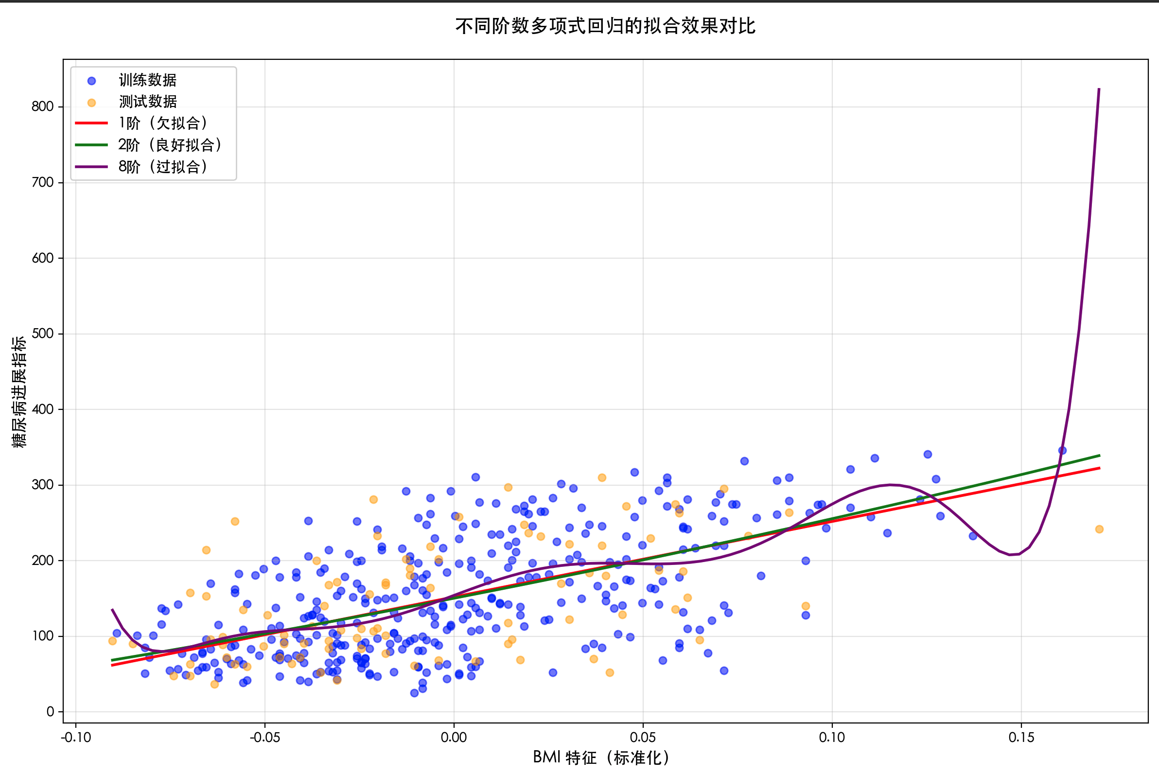
How to interpret learning curves?
| Fitting state | Training error | Validation error | Curve characteristics |
|---|---|---|---|
| Underfitting | High | High | Both curves are high and very close; adding data does not help. |
| Good fitting | Low | Low | Both curves are low and close to each other, reaching a balance point. |
| Overfitting | Very low | High | Training error is very low, but validation error is high, with an obvious gap in between. Adding data usually brings them closer. |
2. Countermeasures
Based on the diagnosis results, we can adopt different strategies:
Addressing underfitting (high bias):
- Increase model complexity: Use more powerful models (e.g., switch from linear models to tree models, neural networks).
- Add more features: Mine or construct more meaningful features.
- Reduce regularization: If regularization (e.g., L1, L2) is used, try to weaken its strength.
- Extend training time: For iterative models (e.g., neural networks), train for more epochs.
Addressing overfitting (high variance):
- Get more training data: One of the most effective methods.
- Reduce model complexity: Choose a simpler model (e.g., lower polynomial degree, reduce tree depth, reduce number of neural network layers).
- Feature selection: Remove irrelevant or redundant features.
- Increase regularization:
- L1 regularization (Lasso): Tends to produce sparse weights and can be used for feature selection.
- L2 regularization (Ridge): Causes weight decay, tending to make all weights small.
- Dropout(for neural networks): Randomly "drop" a portion of neurons during training.
- Early stopping(for iterative models): Stop training when validation error no longer decreases.
IV. Hands-On Practice: Experience with Real Datasets
Let's practice on the classic Boston housing dataset (or the diabetes dataset, since the Boston dataset has been deprecated).
Example
import matplotlib.pyplot as plt
from sklearn.datasets import load_diabetes
from sklearn.model_selection import train_test_split
from sklearn.tree import DecisionTreeRegressor
from sklearn.metrics import mean_squared_error
# -------------------------- Configure Chinese font start --------------------------
plt.rcParams['font.sans-serif'] = [
# Windows first
'SimHei', 'Microsoft YaHei',
# macOS first
'PingFang SC', 'Heiti TC',
# Linux first
'WenQuanYi Micro Hei', 'DejaVu Sans'
]
# Fix the issue of negative signs displaying as blocks
plt.rcParams['axes.unicode_minus'] = False
# -------------------------- Configure Chinese font end --------------------------
# Load data
data = load_diabetes()
X, y = data.data, data.target
X_train, X_test, y_train, y_test = train_test_split(X, y, test_size=0.2, random_state=42)
# Try decision trees with different complexities
max_depths = [1, 3, 10, None] # None means no depth limit; the tree keeps growing until "pure"
train_errors = []
test_errors = []
for depth in max_depths:
model = DecisionTreeRegressor(max_depth=depth, random_state=42)
model.fit(X_train, y_train)
y_train_pred = model.predict(X_train)
y_test_pred = model.predict(X_test)
train_error = mean_squared_error(y_train, y_train_pred)
test_error = mean_squared_error(y_test, y_test_pred)
train_errors.append(train_error)
test_errors.append(test_error)
print(f"Max tree depth: {depth if depth is not None else 'Unlimited'}")
print(f" Training set MSE: {train_error:.2f}")
print(f" Test set MSE: {test_error:.2f}")
print("-" * 30)
# Visualization
plt.figure(figsize=(10, 6))
depths = [str(d) if d else 'Unlimited' for d in max_depths]
x_index = np.arange(len(depths))
width = 0.35
plt.bar(x_index - width/2, train_errors, width, label='Training error', color='skyblue')
plt.bar(x_index + width/2, test_errors, width, label='Test error', color='lightcoral')
plt.xlabel('Maximum decision tree depth (model complexity)')
plt.ylabel('Mean squared error (MSE)')
plt.title('Bias-variance tradeoff: performance of decision trees with different complexity')
plt.xticks(x_index, depths)
plt.legend()
plt.grid(True, axis='y')
plt.tight_layout()
plt.show()
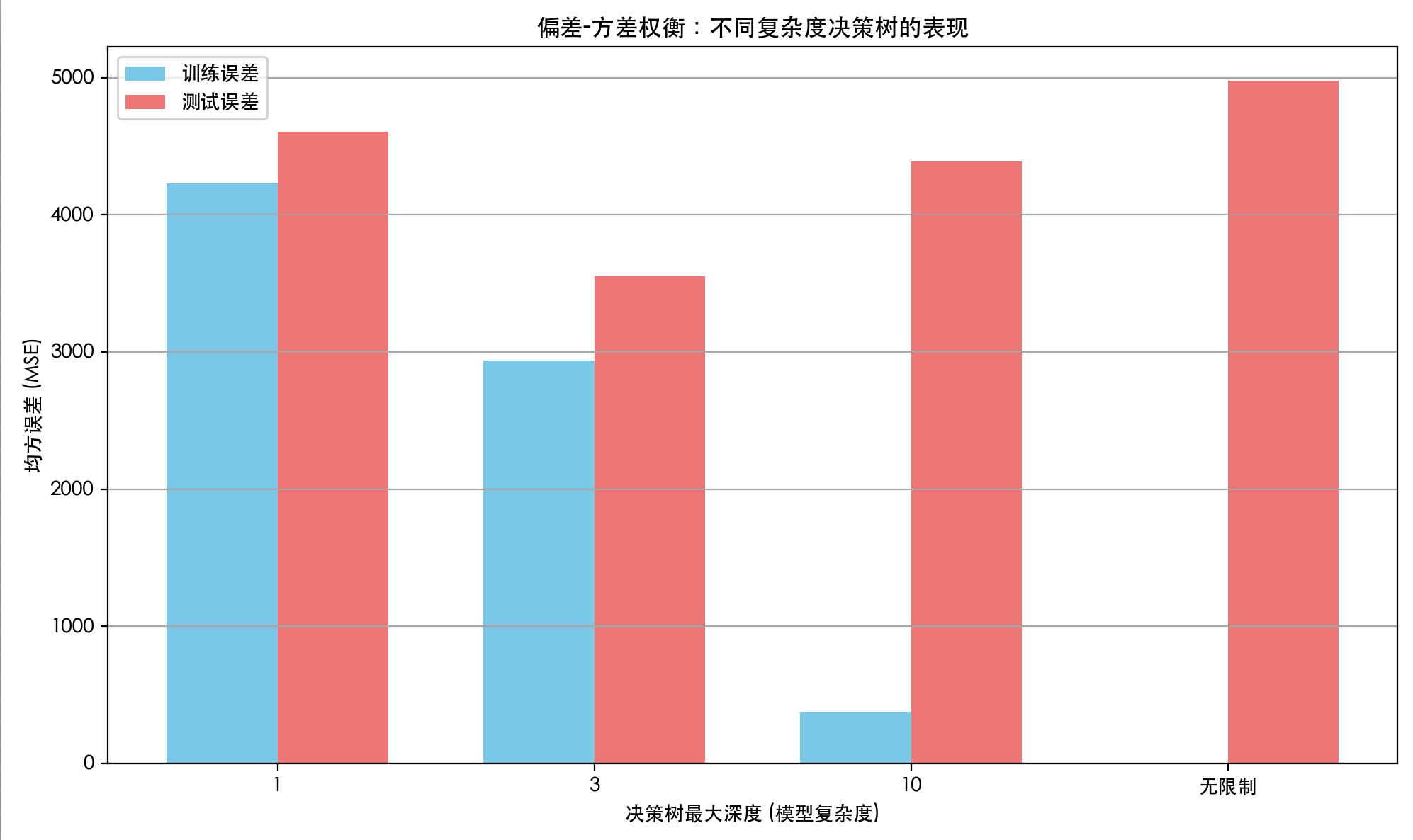
Analysis results:
- Depth=1: The model is very simple, both training and test errors are high ->high bias, underfitting。
- Depth=3: Model complexity increases, both errors decrease significantly and are relatively close ->Bias-variance balance, good fit。
- Depth=10 or unlimited: The model is very complex, training error is extremely low, but test error starts to rise (or is much higher than training error) ->High variance, overfitting。
Summary
Understanding overfitting, underfitting, bias and variance is the cornerstone of building excellent machine learning models. Remember this core loop:
- Train the model -> Evaluate its performance on the training and validation sets。
- Diagnose problems through learning curves or error comparison: Is it high bias (underfitting) or high variance (overfitting)?
- Apply the corresponding strategy(increase complexity/data, regularization, etc.) to improve.
- Return to step 1, until a satisfactory model with strong generalization ability is obtained on the validation set.