Statistics Basics
Before learning various cool algorithms, we need to first lay a crucial foundation—statistics。
We can think of statistics as thelanguageandtoolbox, without it, machine learning models are like explorers without a map, unable to understand data, make predictions, or evaluate their own performance.
This article will systematically introduce the core statistical concepts essential to machine learning, using plain language and vivid examples to help you build a solid theoretical foundation.
Why does machine learning need statistics?
Core reason: Machine learning is essentiallylearning patterns from data, and using this pattern forpredictionorand decision-making.And statistics, precisely, is the science of how to collect, analyze, interpret, and present data.
- Data Understanding: Statistics helps us describe the basic characteristics of data (e.g., average height, income distribution). This is the first step in data cleaning and exploration.
- Pattern Mining: It provides methods for inferring general patterns (models) from data, and tells us how reliable these patterns are.
- Prediction and Evaluation: Statistical theory underpins how we use models to make predictions, and how to objectively evaluate a model’s quality (is it guessing blindly or truly understanding?).
- Uncertainty Quantification: The real world is full of noise; statistics allows us to quantify the uncertainty in predictions (e.g., "I am 95% confident that it will rain tomorrow").
In simple terms,statistics is the theoretical cornerstone of machine learning, transforming intelligence from mysticism into science.
Core Concept 1: Descriptive Statistics
Descriptive statistics is like taking a snapshot and a health check report of data, using a few key metrics to summarize the overall picture of a dataset. This is the starting point of any data analysis project.
1. Central Tendency: Where does the data cluster?
These metrics tell us where the center or typical value of the data lies.
| Metric | Explanation (metaphor) | Calculation formula (brief) | Features and uses |
|---|---|---|---|
| Mean | The arithmetic average of all data. Like the "average salary." |
Sum / Number of data points |
Most commonly used, but very sensitive to extreme values (e.g., billionaires) and easily "averaged up." |
| Median | After sorting the data from smallest to largest,the exact middlevalue. Like the "median salary." |
Take the value at the middle position after sorting. | Robust, unaffected by extreme values, and better reflects typical situations. |
| Mode | The value that appearsmost frequentlyin the data. Like the best-selling shoe size in a store. |
The value with the highest frequency | Suitable for categorical data, or for finding the most common category. |
Example: The monthly salaries (in thousands of yuan) of 5 employees in a department are:[30, 35, 40, 45, 200](The boss is among them.)
- Mean = (30+35+40+45+200)/5 = 70. This value is artificially high because of the boss’s 200 and cannot represent employee income.
- Median= the third number after sorting40. This value better represents the income of a "typical" employee in the department.
- Mode= all values appear only once, sothere is no mode.。
2. Dispersion: How spread out is the data?
Knowing the center alone is not enough; we also need to know whether the data is tightly clustered around the center or scattered widely. Dispersion measures the volatility or diversity of the data.
| Metric | Explanation (metaphor) | Calculation formula (brief) | Features and uses |
|---|---|---|---|
| Variance | The distance of each data point from the mean,squared,is averaged. | Σ(每个值 - 均值)² / (n-1) |
Measures overall dispersion; the unit is the square of the original unit. |
| Standard Deviation | The positive square root of the variance.。 Like the "average fluctuation range." |
√Variance |
Most commonly used, with the same unit as the original data, intuitively reflecting the magnitude of fluctuation. The larger the value, the more dispersed the data. |
| Range | The difference between the maximum and minimum values. "Salary span." |
Maximum value - Minimum value |
Simple to calculate, but determined only by two extreme values, easily affected by outliers. |
Continuing the example above: Calculate the standard deviation of employee salaries (using 40 as the estimated mean is more reasonable).
- Calculate the variance:
[(30-40)² + (35-40)² + (40-40)² + (45-40)² + (200-40)²] / 4 ≈ 5875 - Standard deviation =
√5875 ≈ 76.65. This huge standard deviation (76.65) is far larger than the mean (40),strongly indicating that there is an extreme outlier in the data (the boss’s 200), requiring further analysis.
3. Data Distribution and Visualization
Numeric metrics are abstract; charts allow us to intuitively "see" the data.
- Histogram: Shows the frequency distribution of data within different intervals (bins). It reveals whether the data is unimodal or multimodal, and whether it is symmetric.
- Box plot: Uses a "box" and "whiskers" to display the data’sminimum, first quartile (Q1), median (Q2), third quartile (Q3), and maximum, and is a powerful tool for identifyingoutliers.
Example
import matplotlib.pyplot as plt
import seaborn as sns
import numpy as np
# Employee salary data, containing one outlier
salaries = np.array([30, 35, 40, 45, 200])
employee_names = ['Alice', 'Bob', 'Charlie', 'Diana', 'Boss']
plt.figure(figsize=(8, 5))
# Create a box plot
sns.boxplot(y=salaries)
plt.title('Department Salary Distribution (Boxplot)')
plt.ylabel('Salary (k)')
plt.grid(axis='y', linestyle='--', alpha=0.7)
# Mark the point corresponding to the outlier
for i, (name, salary) in enumerate(zip(employee_names, salaries)):
if salary > 45 + 1.5 * (45-35): # Simple rule for outlier detection
plt.annotate(f'{name}: {salary}', xy=(0, salary), xytext=(0.2, salary),
arrowprops=dict(facecolor='red', shrink=0.05))
plt.show()
Code explanation:
sns.boxplot()Draw a box plot. The box spans from Q1 to Q3, and the middle line is the median.- The "whiskers" of a box plot typically extend to the farthest data point within 1.5 times the interquartile range (IQR = Q3 - Q1); points beyond this are consideredoutliersand are separately marked with dots. In the figure,
200this point is clearly identified as an outlier.
Core Concept 2: Probability and Distributions
If descriptive statistics is about looking at history, then probability is about predicting the future. It quantifiesthe likelihood of an event occurring.。
1. Basic Probability
- Probability P(A): The likelihood of event A occurring, ranging from 0 (impossible) to 1 (certain).
- Conditional Probability P(A|B): Under the condition that event Bhas occurred, the probability of event A occurring. This is key to understanding many machine learning algorithms (such as Naive Bayes).
- Formula:
P(A|B) = P(A 且 B) / P(B)
- Formula:
2. Probability Distributions
Describes the probability rules of a random variable taking on various possible values. The most important one in machine learning is:
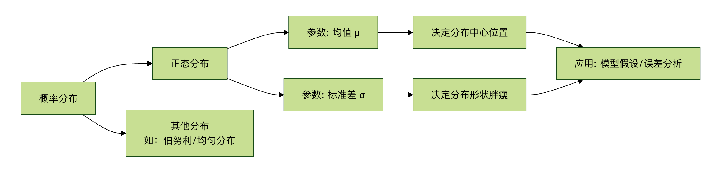
- Normal Distribution (Gaussian Distribution):
- Shape: The famous "bell curve," symmetric left and right.
- Parameters: The **mean (μ)** determines the center position, and the **standard deviation (σ)** determines the "thickness" (dispersion) of the curve.
- Importance: Many phenomena in nature and social science approximately follow a normal distribution (e.g., height, measurement errors). The central limit theorem states that the sum of many independent random variables tends toward a normal distribution, making it the cornerstone of statistical inference.
- 68-95-99.7 Rule: The probabilities that data fall within mean ±1σ, ±2σ, and ±3σ are approximately 68%, 95%, and 99.7%, respectively.
Core Concept 3: Inferential Statistics
This is the "advanced version" of statistics; the goal is fromsampledata to inferpopulationproperties.
1. Central Limit Theorem
Core idea: No matter what the population distribution is, when we draw a large number ofindependentrandom samples from the population, and calculate themeanof each sample, the distribution of these sample means will tend toward anormal distribution.。
Significance for machine learning: This allows us to use the properties of the normal distribution to performhypothesis testingand constructconfidence intervalson model parameters (such as the mean), providing a theoretical basis. Even if we do not know the true distribution of the population, we can analyze the reliability of estimates based on samples.
2. Hypothesis Testing
It is used to determine whether a hypothesis about the population (such as "the new drug is ineffective") is supported by the sample data.
- Null hypothesis (H0): Usually means "no effect" or "no difference" (default position).
- Alternative hypothesis (H1): The hypothesis we want to confirm (e.g., "the new drug is effective").
- P-value: The probability of observing the current sample data (or more extreme data) assuming the null hypothesis is true.
- How to decide: If the P-value is very small (usually < 0.05), it means the current situation is extremely unlikely under H0, so we have sufficient evidence toreject H0and accept H1.
- Significance level (α): The threshold used to determine whether the P-value is "small enough", often set to 0.05.
Applications in machine learning: Used for feature selection to determine whether a statistically significant correlation exists between a feature and the target variable, rather than a coincidental association.
3. Correlation and Causation
This is one of the most easily confused and most important concepts in data analysis.
- Correlation: Measures the tendency of two variables tochange together. It is often represented by the **correlation coefficient (ranging from -1 to 1)**.
- 1: Perfect positive correlation (increase and decrease together).
- -1: Perfect negative correlation (one increases while the other decreases).
- 0: No linear correlation.
- Causation: Refers to a variable (cause) whosechange directly leads tothe change of another variable (effect).
Key difference:Correlation does not equal causation!
- Classic fallacy: Ice cream sales and drowning incidents are highly positively correlated in summer. But this does not mean eating ice cream causes drowning. Theircommon cause (confounding variable)Yesis the hot weather.。
- Implications for machine learning: Machine learning models (especially predictive models) excel at discoveringcorrelation, but cannot determine on their owncausation. Mistaking strong correlations found by models for causal relationships is a common mistake in practice. Establishing causal models requires more rigorous experimental designs (e.g., randomized controlled trials) or special causal inference methods.
Hands-on Practice: Basic Statistical Analysis with Python
Let's use Python and the well-knownpandas、seabornlibrary to perform simple descriptive and exploratory statistical analysis on a real dataset.
Example
import seaborn as sns
import matplotlib.pyplot as plt
import numpy as np
# 1. Load the dataset (using seaborn's built-in 'tips' tip dataset)
df = sns.load_dataset('tips')
print("First 5 rows of the dataset:")
print(df.head())
print(f"\n"Dataset shape: {df.shape}") # View the number of rows and columns
print("\n"Basic information:")
print(df.info())
print("\n"Descriptive statistics:")
print(df.describe())
# 2. Explore the numerical variables: total bill (total_bill) and tip (tip)
print(f"\n"Mean total bill: {df['total_bill'].mean():.2f}")
print(f"Median total bill: {df['total_bill'].median():.2f}")
print(f"Standard deviation of total bill: {df['total_bill'].std():.2f}")
print(f"Correlation coefficient between tip and total bill: {df['tip'].corr(df['total_bill']):.3f}")
# 3. Visualization
fig, axes = plt.subplots(2, 2, figsize=(12, 10))
# 3.1 Histogram and density estimate of total bill
sns.histplot(df['total_bill'], kde=True, ax=axes[0, 0])
axes[0, 0].set_title('Distribution of Total Bill')
axes[0, 0].axvline(df['total_bill'].mean(), color='red', linestyle='--', label=f'Mean: {df["total_bill"].mean():.1f}')
axes[0, 0].axvline(df['total_bill'].median(), color='green', linestyle='--', label=f'Median: {df["total_bill"].median():.1f}')
axes[0, 0].legend()
# 3.2 Scatter plot of tip vs. total bill (to examine correlation)
sns.scatterplot(data=df, x='total_bill', y='tip', hue='time', ax=axes[0, 1])
axes[0, 1].set_title('Tip vs Total Bill (Colored by Meal Time)')
# 3.3 Box plot of tip grouped by sex (to compare differences between groups)
sns.boxplot(data=df, x='sex', y='tip', ax=axes[1, 0])
axes[1, 0].set_title('Tip Amount by Gender')
# 3.4 Bar chart of mean bill by smoking status
bill_by_smoker = df.groupby('smoker')['total_bill'].mean().reset_index()
sns.barplot(data=bill_by_smoker, x='smoker', y='total_bill', ax=axes[1, 1])
axes[1, 1].set_title('Average Total Bill by Smoking Status')
for index, row in bill_by_smoker.iterrows():
axes[1, 1].text(index, row['total_bill']+0.5, f"{row['total_bill']:.1f}", ha='center')
plt.tight_layout()
plt.show()
Practice tasks:
Run the code: Run the above code in your Python environment, observe the outputs and charts.
Interpret the results:
- From the descriptive statistics table, can you tell the approximate range and median of the total bill?
- Are tip and total bill positively or negatively correlated? Can you tell from the scatter plot?
- From the box plot, is there a significant difference in the median tip given by males and females?
Formulate a hypothesis: Based on the bar chart of mean bill by smoking status, can you propose a null hypothesis forhypothesis testing? (For example: H0: There is no difference in the average bill between smokers and non-smokers).
Other extensions