Machine Learning - Customer Segmentation
In today's data-driven business world, understanding customers is the key to success.
However, when your customer base reaches tens of thousands or even millions, manually analyzing each customer's characteristics and behavioral patterns becomes impractical.
At this point, machine learning techniques, especiallyunsupervised learningclustering algorithms within it, become a powerful tool.
Customer segmentation, also known as customer segmentation, has the core goal of dividing the large customer base into several subgroups with similar characteristics. This is like an experienced store owner who no longer treats customers as a vague whole, but can clearly identify different groups such as value-conscious homemakers, tech enthusiasts keen on new products, and high-end customers who value service experience. By adopting targeted marketing, service, and product strategies for different groups, companies can significantly improve operational efficiency and customer satisfaction.
This article will guide you step by step through a complete customer segmentation hands-on project. We will use the classic K-Means clustering algorithm to analyze a simulated retail customer dataset, from data understanding to model evaluation, ultimately obtaining segmentation results with business insights.
Understanding Cluster Analysis and K-Means Algorithm
Before starting the hands-on practice, we need to understand the core tools we are about to use.
What is Cluster Analysis?
Cluster analysis is an unsupervised learning method. Unlike supervised learning (such as predicting house prices or identifying cat and dog images), clustering algorithms do not have pre-labeled "correct answers" (i.e., labels). Its task is to explore the inherent structure of data, automatically grouping similar data points into the same group (called a "cluster"), while making data points in different groups as dissimilar as possible.
A simple analogy: Imagine you have a basket of mixed fruits containing apples, oranges, and bananas. The task of the clustering algorithm is to automatically pile together fruits that are similar in shape, color, and size without anyone telling you the category names.
How the K-Means Algorithm Works
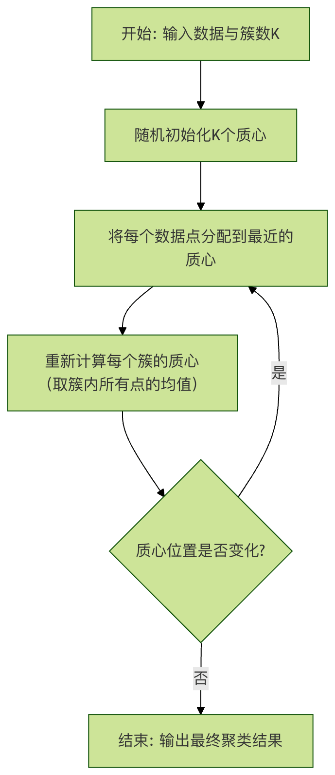
K-Means is one of the most commonly used and intuitive clustering algorithms. "K" represents the number of clusters we want to divide the data into. Its working principle can be summarized in four steps:
- Initialization: Randomly select K data points as the initial "cluster centers" (centroids).
- Assignment: Calculate the distance from each data point to each centroid (usually using Euclidean distance), then assign each point to the cluster of the nearest centroid.
- Update: Recalculate the centroid of each cluster (i.e., the mean of all points in that cluster).
- Iteration: Repeat steps 2 and 3 until the positions of the centroids no longer change significantly, or the preset number of iterations is reached.
The flowchart below clearly illustrates this process:
Algorithm Core Points:
- Distance Metric: Usually, Euclidean distance is used to measure the similarity between data points; the closer the distance, the higher the similarity.
- Centroid: Represents the "average point" or center of a cluster.
- Objective: Minimize the sum of squared distances from data points to their centroid within each cluster (called "within-cluster sum of squares" or Inertia).
Hands-on Practice: Retail Customer Segmentation
Now, let's put theory into practice. We will use Python and its powerful data science ecosystem libraries to complete this project.
Step 1: Environment Setup and Data Loading
First, ensure that the necessary libraries are installed in your Python environment:pandasfor data processing,numpyfor numerical computation,matplotlibandseabornfor visualization,scikit-learnis the core machine learning library.
Example
import pandas as pd
import numpy as np
import matplotlib.pyplot as plt
import seaborn as sns
from sklearn.cluster import KMeans
from sklearn.preprocessing import StandardScaler
from sklearn.metrics import silhouette_score
import warnings
warnings.filterwarnings('ignore') # Ignore non-critical warnings
# Set visualization style
sns.set_style("whitegrid")
# -------------------------- Set Chinese font start --------------------------
plt.rcParams['font.sans-serif'] = [
# Windows first
'SimHei', 'Microsoft YaHei',
# macOS first
'PingFang SC', 'Heiti TC',
# Linux first
'WenQuanYi Micro Hei', 'DejaVu Sans'
]
# Fix the issue of negative signs displaying as squares
plt.rcParams['axes.unicode_minus'] = False
# -------------------------- Set Chinese font end --------------------------
We will use a simulated customer datasetcustomer_data.csv, which typically contains the following features:
CustomerID: Customer unique identifierAnnual_Income_(k$): Customer annual income (thousands of dollars)Spending_Score: Spending score (0-100, comprehensively derived from purchase frequency, amount, etc.)Age: Age
The content is as follows:
CustomerID,Age,Annual_Income_(k$),Spending_Score
1,19,15,39
2,21,15,81
3,20,16,6
4,23,16,77
5,31,17,40
6,22,17,76
7,35,18,6
8,23,18,94
9,64,19,3
10,30,19,72
11,67,20,14
12,35,20,99
13,58,21,15
14,24,21,77
15,37,22,13
16,22,22,79
17,35,23,35
18,20,23,66
19,52,24,29
20,35,24,98
21,46,25,35
22,25,25,73
23,54,26,5
24,28,26,73
25,45,27,28
26,23,28,82
27,40,28,36
28,35,28,61
29,60,29,4
30,21,30,87
31,62,30,17
32,23,30,73
33,18,31,92
34,49,33,14
35,21,33,81
36,42,34,17
37,30,34,73
38,36,37,26
39,20,37,75
40,65,38,35
41,24,38,92
42,48,39,36
43,31,39,61
44,49,40,29
45,24,40,98
46,50,41,15
47,27,42,65
48,29,43,88
49,31,43,19
50,49,44,75
Example
df = pd.read_csv('customer_data.csv')
print("Data shape (rows, columns):", df.shape)
print("\n"First 5 rows of data:")
print(df.head())
print("\n"Data basic information:")
print(df.info())
print("\n"Descriptive statistics:")
print(df.describe())
Output:
数据形状(行数,列数): (50, 4)

数据前5行:
   CustomerID  Age  Annual_Income_(k$)  Spending_Score
0           1   19                  15              39
1           2   21                  15              81
2           3   20                  16               6
3           4   23                  16              77
4           5   31                  17              40

数据基本信息:
<class 'pandas.core.frame.DataFrame'>
RangeIndex: 50 entries, 0 to 49
Data columns (total 4 columns):
 #   Column              Non-Null Count  Dtype
---  ------              --------------  -----
 0   CustomerID          50 non-null     int64
 1   Age                 50 non-null     int64
 2   Annual_Income_(k$)  50 non-null     int64
 3   Spending_Score      50 non-null     int64
dtypes: int64(4)
memory usage: 1.7 KB
None

描述性统计:
       CustomerID        Age  Annual_Income_(k$)  Spending_Score
count    50.00000  50.000000           50.000000       50.000000
mean     25.50000  35.560000           28.160000       51.680000
std      14.57738  14.283085            8.739682       31.506682
min       1.00000  18.000000           15.000000        3.000000
25%      13.25000  23.000000           21.000000       20.750000
50%      25.50000  31.000000           27.500000       61.000000
75%      37.75000  47.500000           36.250000       77.000000
max      50.00000  67.000000           44.000000       99.000000
Step 2: Data Exploration and Preprocessing
Before applying the algorithm, we must first understand the data and do the "cleaning" work properly.
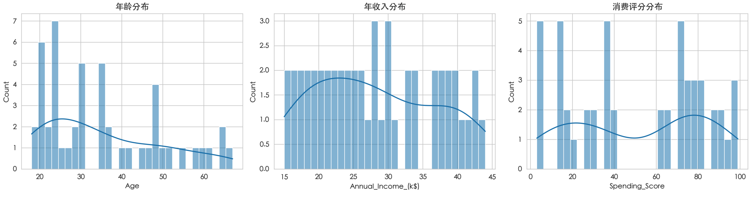
1. Exploratory Data AnalysisDiscover patterns initially through visualization and statistics.
Example
fig, axes = plt.subplots(1, 3, figsize=(15, 4))
sns.histplot(df['Age'], bins=30, kde=True, ax=axes[0])
axes[0].set_title('Age Distribution')
sns.histplot(df['Annual_Income_(k$)'], bins=30, kde=True, ax=axes[1])
axes[1].set_title('Annual Income Distribution')
sns.histplot(df['Spending_Score'], bins=30, kde=True, ax=axes[2])
axes[2].set_title('Spending Score Distribution')
plt.tight_layout()
plt.show()
# View relationships between features
sns.pairplot(df[['Age', 'Annual_Income_(k$)', 'Spending_Score']])
plt.suptitle('Feature Relationship Scatter Plot Matrix', y=1.02)
plt.show()
2. Data PreprocessingClustering algorithms are very sensitive to the dimension (units) of features. The numerical ranges of annual income (tens of thousands) and age (tens) differ greatly, which will seriously affect distance calculation and cause the income feature to dominate the clustering results. Therefore, we need to performfeature standardization, which scales each feature to a standard normal distribution with mean 0 and variance 1.
Example
features = ['Age', 'Annual_Income_(k$)', 'Spending_Score']
X = df[features].copy()
# Feature standardization
scaler = StandardScaler()
X_scaled = scaler.fit_transform(X) # fit calculates mean and variance, transform applies the transformation
X_scaled_df = pd.DataFrame(X_scaled, columns=features)
print("First 5 rows of standardized data:")
print(X_scaled_df.head())
Step 3: Determining the Optimal Number of Clusters (K Value)
K-Means requires us to specify the K value in advance. How to choose a reasonable K? We use two classic methods:
1. Elbow MethodPlot the within-cluster sum of squares (Inertia) corresponding to different K values. Inertia decreases as K increases; we look for the inflection point of the curve (like an elbow), after which the benefit (decrease in Inertia) from further increasing K becomes smaller.
Example
K_range = range(1, 11) # Test K from 1 to 10
for k in K_range:
kmeans = KMeans(n_clusters=k, random_state=42, n_init='auto') # n_init='auto' is a usage in newer versions
kmeans.fit(X_scaled)
inertia.append(kmeans.inertia_) # Get the Inertia under this K value
# Plot the elbow method graph
plt.figure(figsize=(8,5))
plt.plot(K_range, inertia, 'bo-')
plt.xlabel('Number of Clusters (K)')
plt.ylabel('Within-cluster Sum of Squares (Inertia)')
plt.title('Elbow Method: Choosing the Best K Value')
plt.xticks(K_range)
plt.show()
2. Silhouette Coefficient MethodThe silhouette coefficient measures the similarity of a data point to its own cluster (cohesion) and its separation from other clusters. Its value ranges from -1 to 1,the higher the better, indicating better clustering performance.
Example
K_range = range(2, 11) # The silhouette coefficient requires at least 2 clusters
for k in K_range:
kmeans = KMeans(n_clusters=k, random_state=42, n_init='auto')
cluster_labels = kmeans.fit_predict(X_scaled)
score = silhouette_score(X_scaled, cluster_labels)
silhouette_scores.append(score)
# Plot the silhouette coefficient graph
plt.figure(figsize=(8,5))
plt.plot(K_range, silhouette_scores, 'go-')
plt.xlabel('Number of Clusters (K)')
plt.ylabel('Silhouette Coefficient')
plt.title('Silhouette Coefficient Method: Choosing the Best K Value')
plt.xticks(K_range)
plt.show()
Combining the elbow method graph (inflection point) and the silhouette coefficient graph (peak), we assume and determineK=5is a good choice.
Step 4: Applying K-Means for Clustering
Train the model using the selected K value and assign cluster labels to each customer.
Example
final_k = 5
kmeans_final = KMeans(n_clusters=final_k, random_state=42, n_init='auto')
df['Cluster'] = kmeans_final.fit_predict(X_scaled) # Add cluster labels to the original dataframe
# View the number of customers in each cluster
cluster_counts = df['Cluster'].value_counts().sort_index()
print("Distribution of customer counts per cluster:")
print(cluster_counts)
# View feature means per cluster (original scale)
cluster_profile = df.groupby('Cluster')[features].mean().round(2)
print("\nAverage feature values per cluster:)
print(cluster_profile)
Step 5: Result Analysis and Visualization
Transform abstract cluster labels into intuitive insights.
1. Visualize the clustering resultsSince we have three features, we can select the two most important features (e.g., income and spending score) for visualization on a two-dimensional plane.
Example
plt.figure(figsize=(10, 6))
scatter = plt.scatter(df['Annual_Income_(k$)'], df['Spending_Score'],
c=df['Cluster'], cmap='viridis', s=50, alpha=0.7)
plt.colorbar(scatter, label='Cluster label')
plt.xlabel('Annual Income (k$)')
plt.ylabel('Spending Score')
plt.title('Customer segmentation results (based on annual income and spending score)')
plt.show()
2. Profile customer segmentsAccording tocluster_profilethe table, we can assign business meaning to each cluster:
| Cluster label | Age | Annual income | Spending score | Possible customer profile |
|---|---|---|---|---|
| 0 | Medium | High | Low | High-income cautious type: High income but conservative spending; may be savers or high-net-worth individuals who are price-sensitive. |
| 1 | Medium | Low | Low | Low-income low-spending type: Both income and spending power are limited; they need cost-effective products. |
| 2 | Medium | Low | High | Value-seeking type: Income is not high but they love to spend; they value trends and experiences, and are targets for promotional activities. |
| 3 | Medium | High | High | Ideal VIP type: High income and high spending; they are the core profit source of the enterprise and should be provided with top-tier services and exclusive benefits. |
| 4 | Young | Medium | Medium | Young potential type: Young customers whose income and spending are in a growth stage; they are key to cultivating brand loyalty. |
Step 6: Model Evaluation and Application Recommendations
Evaluation: In addition to the silhouette score, you can check whether the sample distribution within clusters is balanced, and combine business logic to judge whether the segmentation is reasonable.
Application Recommendations:
- Precision marketing: Push high-end new products and exclusive events to the "Ideal VIP type" (Cluster 3); send discount coupons and group-buying information to the "Value-seeking type" (Cluster 2).
- Product development: Design fashionable products with strong social attributes for the "Young potential type" (Cluster 4).
- Customer service: Provide detailed product data and security guarantees to the "High-income cautious type" (Cluster 0) to alleviate their concerns.
- Resource allocation: Allocate more customer service and marketing resources to high-value customer segments.
Summary and Further Exploration
Through this hands-on case, you have fully experienced the process of customer segmentation using the K-Means algorithm:Data preparation -> Exploratory analysis -> Preprocessing -> Determine K value -> Train model -> Analyze results。
Key Points Review:
- Clustering is an unsupervised learning method used to discover inherent groupings in data.
- Feature standardizationis a key step before using distance-based clustering algorithms.
- Elbow methodandSilhouette scoreare practical tools for determining the optimal number of clusters.
- The interpretation of clustering results mustbe combined with business knowledgeto produce real value.