Linear Regression
Linear Regression is one of the most fundamental and widely used algorithms in machine learning.
Linear Regression is the most basic machine learning algorithm for predicting continuous values; it assumes that the target variableyand the feature variablesxhave a linear relationship, and tries to find a best-fit line to describe this relationship.
y = w * x + b
Where:
yis the predicted valuexis the feature variablewis the weight (slope)bis the bias (intercept)
The goal of linear regression is to find the optimalwandb, so that the predicted valueyhas the minimum error from the true value. The commonly used error function is the Mean Squared Error (MSE):
MSE = 1/n * Σ(y_i - y_pred_i)^2
Where:
- y_i is the actual value.
- y_pred_i is the predicted value.
- n is the number of data points.
Our goal is to minimize MSE by adjusting w and b.
How to solve linear regression?
1. Least Squares Method
The least squares method is a common approach to solving linear regression; it finds the optimal (w) and (b) by solving the following equations.
The goal of the least squares method is to minimize the Residual Sum of Squares (RSS), with the formula:
\[ \text{RSS} = \sum_{i=1}^n (y_i - \hat{y}_i)^2 \]
Where:
\( y_i \)is the actual value.\( \hat{y}_i \)is the predicted value, which is\( \hat{y}_i = w x_i + b \)calculated by the linear regression model.
By minimizing RSS, the following normal equations can be obtained:
\[ \begin{cases} w \sum_{i=1}^n x_i^2 + b \sum_{i=1}^n x_i = \sum_{i=1}^n x_i y_i \\ w \sum_{i=1}^n x_i + b n = \sum_{i=1}^n y_i \end{cases} \]
Matrix form
Write the normal equations in matrix form:
\[ \begin{bmatrix} \sum_{i=1}^n x_i^2 & \sum_{i=1}^n x_i \\ \sum_{i=1}^n x_i & n \end{bmatrix} \begin{bmatrix} w \\ b \end{bmatrix} = \begin{bmatrix} \sum_{i=1}^n x_i y_i \\ \sum_{i=1}^n y_i \end{bmatrix} \]
Solution method
By solving the above matrix equation, the optimal can be obtained.\( w \)and\( b \):
\[ \begin{bmatrix} w \\ b \end{bmatrix} = \begin{bmatrix} \sum_{i=1}^n x_i^2 & \sum_{i=1}^n x_i \\ \sum_{i=1}^n x_i & n \end{bmatrix}^{-1} \begin{bmatrix} \sum_{i=1}^n x_i y_i \\ \sum_{i=1}^n y_i \end{bmatrix} \]
2. Gradient Descent
The goal of gradient descent is to minimize the loss function\( J(w, b) \) . For linear regression problems, the Mean Squared Error (MSE) is usually used as the loss function:
\[ J(w, b) = \frac{1}{2m} \sum_{i=1}^m (y_i - \hat{y}_i)^2 \]
Where:
\( m \)is the number of samples.\( y_i \)is the actual value.\( \hat{y}_i \)is the predicted value, which is\( \hat{y}_i = w x_i + b \)calculated by the linear regression model.
The gradient is the partial derivative of the loss function with respect to the parameters, indicating the direction of change of the loss function in parameter space. For linear regression, the gradient is calculated as follows:
\[ \frac{\partial J}{\partial w} = -\frac{1}{m} \sum_{i=1}^m x_i (y_i - \hat{y}_i) \]
\[ \frac{\partial J}{\partial b} = -\frac{1}{m} \sum_{i=1}^m (y_i - \hat{y}_i) \]
Parameter update rules
Gradient descent updates the parameters using the following rules:\( w \)and\( b \):
\[ w := w - \alpha \frac{\partial J}{\partial w} \]
\[ b := b - \alpha \frac{\partial J}{\partial b} \]
Where:
\( \alpha \)is the learning rate, which controls the step size of each update.
Steps of gradient descent
- Initialize parameters: initialize
\( w \)and\( b \)the values (usually set to 0 or random values). - Compute the loss function: compute the loss function value under the current parameters
\( J(w, b) \)。 - Compute the gradient: compute the partial derivative of the loss function with respect to
\( w \)and\( b \)the parameters. - Update parameters: update according to the gradient
\( w \)and\( b \)。 - Repeat iteration: repeat steps 2 to 4 until the loss function converges or the maximum number of iterations is reached.
Implementing Linear Regression with Python
Below we use a simple example to demonstrate how to implement linear regression using Python.
1. Import necessary libraries
Example
import matplotlib.pyplot as plt
from sklearn.linear_model import LinearRegression
2. Generate simulated data
Example
import matplotlib.pyplot as plt
from sklearn.linear_model import LinearRegression
# Generate some random data
np.random.seed(0)
x = 2 * np.random.rand(100, 1)
y = 4 + 3 * x + np.random.randn(100, 1)
# Visualize the data
plt.scatter(x, y)
plt.xlabel('x')
plt.ylabel('y')
plt.title('Generated Data From Example')
plt.show()
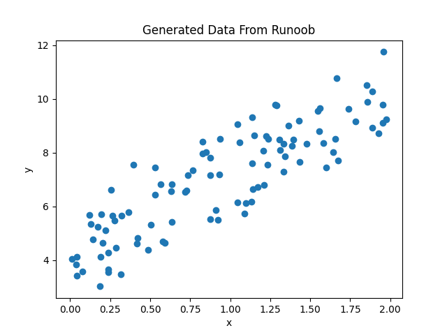
The display is as follows:
3. Using Scikit-learn for Linear Regression
Example
import matplotlib.pyplot as plt
from sklearn.linear_model import LinearRegression
# Generate some random data
np.random.seed(0)
x = 2 * np.random.rand(100, 1)
y = 4 + 3 * x + np.random.randn(100, 1)
# Create a linear regression model
model = LinearRegression()
# Fit the model
model.fit(x, y)
# Output the model parameters
print(f"Slope (w): {model.coef_)
print(f"Intercept (b): {model.intercept_)
# Predict
y_pred = model.predict(x)
# Visualize the fitting result
plt.scatter(x, y)
plt.plot(x, y_pred, color='red')
plt.xlabel('x')
plt.ylabel('y')
plt.title('Linear Regression Fit')
plt.show()
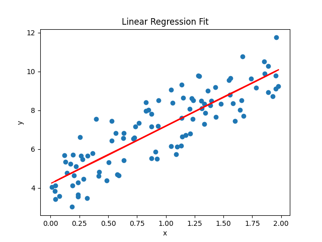
Output result:
斜率 (w): 2.968467510701019
截距 (b): 4.222151077447231
The display is as follows:
We can use thescore()method to evaluate model performance, returning the R^2 value.
Example
from sklearn.linear_model import LinearRegression
# Generate some random data
np.random.seed(0)
x = 2 * np.random.rand(100, 1)
y = 4 + 3 * x + np.random.randn(100, 1)
# Create a linear regression model
model = LinearRegression()
# Fit the model
model.fit(x, y)
# Calculate the model score
score = model.score(x, y)
print("Model score:", score)
The output result is:
模型得分: 0.7469629925504755
4. Implementing Gradient Descent Manually
Example
import matplotlib.pyplot as plt
from sklearn.linear_model import LinearRegression
# Generate some random data
np.random.seed(0)
x = 2 * np.random.rand(100, 1)
y = 4 + 3 * x + np.random.randn(100, 1)
# Initialize parameters
w = 0
b = 0
learning_rate = 0.1
n_iterations = 1000
# Gradient descent
for i in range(n_iterations):
y_pred = w * x + b
dw = -(2/len(x)) * np.sum(x * (y - y_pred))
db = -(2/len(x)) * np.sum(y - y_pred)
w = w - learning_rate * dw
b = b - learning_rate * db
# Output the final parameters
print(f"Manually implemented slope (w): {w}")
print(f"Manually implemented intercept (b): {b}")
# Visualize the manually implemented fitting result
y_pred_manual = w * x + b
plt.scatter(x, y)
plt.plot(x, y_pred_manual, color='green')
plt.xlabel('x')
plt.ylabel('y')
plt.title('Manual Gradient Descent Fit')
plt.show()
Output result:
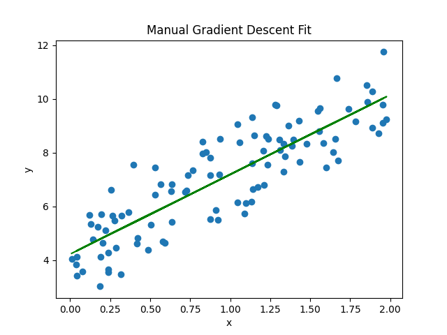
手动实现的斜率 (w): 2.968467510701028
手动实现的截距 (b): 4.222151077447219
The display is as follows: