Forward Propagation and Backpropagation
In deep learning, forward propagation and backpropagation are the two core pillars that support its operation. They are like two sides of the same coin, together forming a complete closed loop from learning to application in neural networks. Thoroughly understanding these two processes is the first key to opening the door to deep learning.
This article will take you step by step through these seemingly complex concepts, using clear logic and vivid analogies, so that you not only know what they are, but also understand why they work.
What are forward propagation and backpropagation?
Before diving into the details, let's first establish a macro-level understanding.
Imagine you are teaching a child to recognize cats and dogs. You show him a picture (input), and based on the knowledge already in his brain (network parameters, i.e., weights and biases) he makes a judgment, then tells you this is a cat (output). This process of looking at the picture -> brain processing -> giving an answer isforward propagation。
But the child's judgment may be wrong. You tell him: no, this is a dog. The difference between the correct answer and the child's answer iserror. The child needs to reflect based on this error: Which knowledge (parameters) in my brain led to this misjudgment? How should I adjust them so I can recognize correctly next time? This process of adjusting knowledge from back to front based on the error isbackpropagation。
In neural networks:
- Forward propagation: The process in which data goes from the input layer, through hidden layers, and finally reaches the output layer, producing a prediction result. This is aninferenceprocess.
- Backpropagation: Based on the error between the prediction result produced by forward propagation and the true value, starting from the output layer, it reversely computes, layer by layer, the "contribution" of each parameter (weight and bias) to the total error (i.e., the gradient), and updates parameters accordingly. This is alearningprocess.
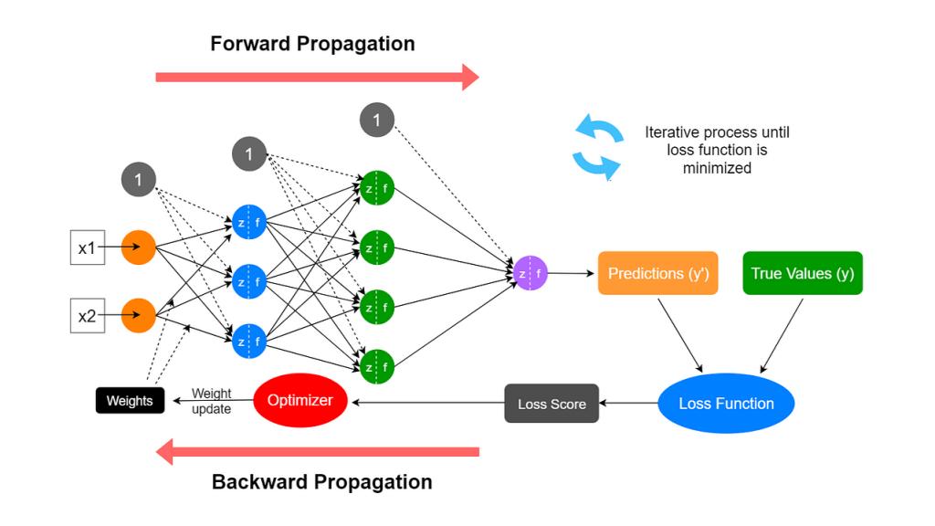
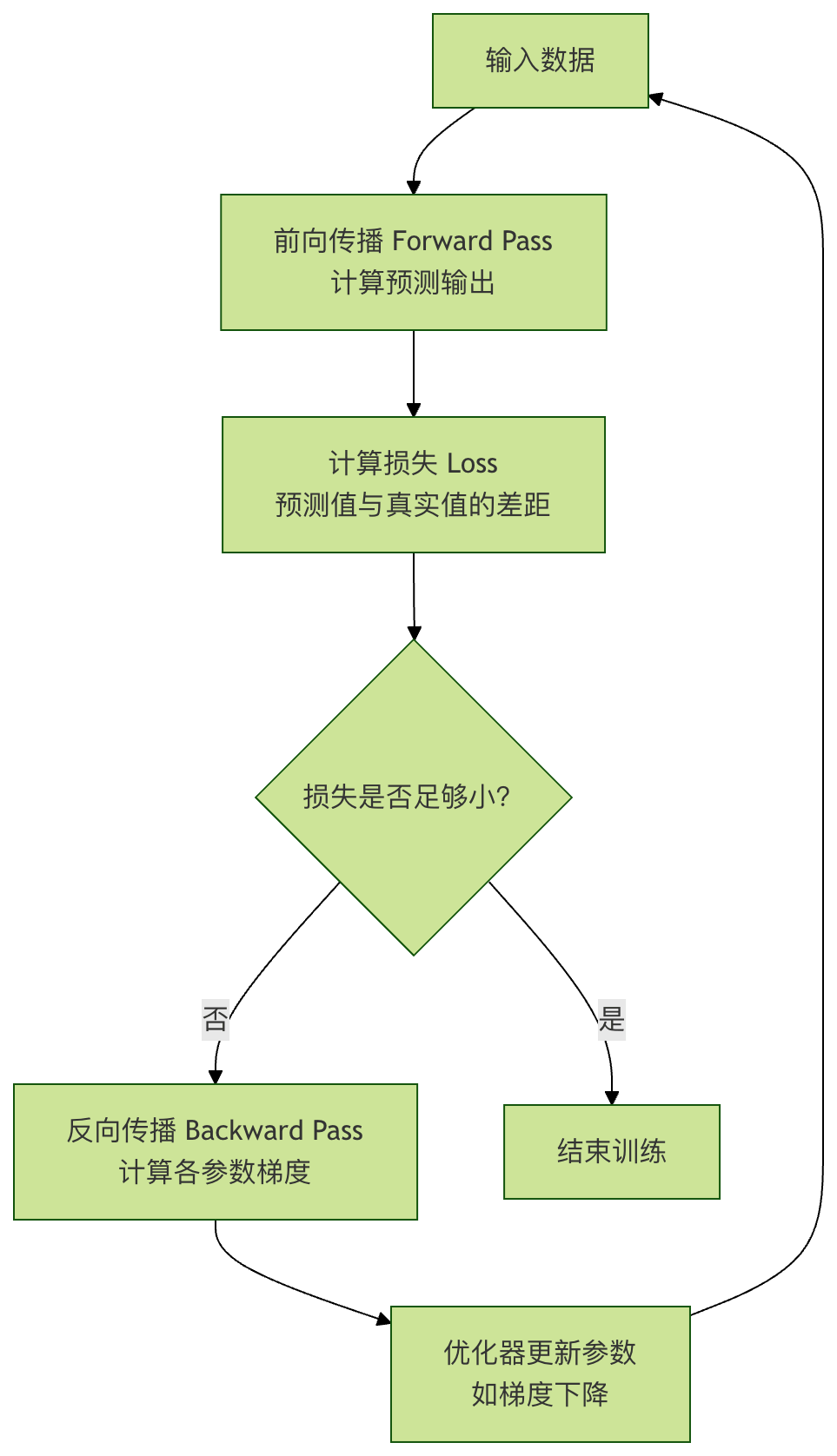
Their relationship can be represented by a simple learning loop diagram:
Forward Propagation: The Inference Path of Neural Networks
Forward propagation is the forward channel through which neural networks make predictions. Let's understand it through a simple three-layer neural network (input layer, one hidden layer, output layer).
Core Concepts and Computation
Suppose we want to predict housing prices, and the input is the house areax. Our miniature network structure is as follows:
- Input layer: one neuron, receiving
x。 - Hidden layer: one neuron, with weight
w1and biasb1。 - Output layer: one neuron, with weight
w2and biasb2, outputting the predicted housing pricey_pred。
The forward propagation computation is divided into two steps:
1. Hidden layer computation: inputxand weightw1, biasb1are combined, then passed through an activation function (e.g., Sigmoid, denoted asσ), producing the hidden layer outputa1。
z1 = w1 * x + b1
a1 = σ(z1) = 1 / (1 + exp(-z1))
z1is the result of the linear transformation.a1is the output after nonlinear activation, which gives the network the ability to learn complex patterns.
2. Output layer computation: hidden layer outputa1as input, with the output layer's weightw2, biasb2are combined to produce the final predictiony_pred. Here for simplicity, assume the output layer does not use an activation function (i.e., linear output).
y_pred = w2 * a1 + b2
Code example: manually implementing forward propagation
Example
def sigmoid(x):
"""Sigmoid activation function"""
return 1 / (1 + np.exp(-x))
# Initialize network parameters (usually random initialization, here specified values for demonstration)
w1, b1 = 2.0, -1.0 # Hidden layer parameters
w2, b2 = 1.5, 0.5 # Output layer parameters
def forward_pass(x):
"""Perform one forward propagation"""
# Hidden layer computation
z1 = w1 * x + b1
a1 = sigmoid(z1) # Apply activation function
# Output layer computation
y_pred = w2 * a1 + b2 # Linear output
# Return intermediate results and final prediction for later understanding
return {'z1': z1, 'a1': a1, 'y_pred': y_pred}
# Assume house area is 3 (unit: 100 square meters)
x_input = 3.0
result = forward_pass(x_input)
print(f"Input x = {x_input}")
print(f"Hidden layer linear output z1 = w1*x + b1 = {result['z1']:.4f}")
print(f"Hidden layer activation output a1 = sigmoid(z1) = {result['a1']:.4f}")
print(f"Final predicted housing price y_pred = w2*a1 + b2 = {result['y_pred']:.4f}")
Example output:
输入 x = 3.0
隐藏层线性输出 z1 = w1*x + b1 = 5.0000
隐藏层激活输出 a1 = sigmoid(z1) = 0.9933
最终预测房价 y_pred = w2*a1 + b2 = 1.9899
Thisy_predis the network's predicted price for a house with area 3. But obviously, this predicted value (based on parameters we set casually) is likely far from the real housing price. How do we measure this gap and improve it? This requiresloss functionand the upcomingbackpropagation。
Loss Function: A Yardstick for Measuring Good or Bad
Before backpropagation begins, we must first quantify the predicted valuey_predand the true valuey_truethe gap between them. This is the role of the loss function.
Common loss functions:
- Mean Squared Error: Suitable for regression problems (e.g., predicting housing prices, temperature).
Loss = (1/N) * Σ (y_true - y_pred)^2 - Cross-Entropy Loss: Suitable for classification problems (e.g., image classification, spam detection).
Taking the mean squared error as an example, for a single sample:
Loss = (y_true - y_pred)^2
Our goal is to adjustw1, b1, w2, b2, to make thisLossvalue as small as possible.
Backpropagation: The Learning Engine of Neural Networks
Backpropagation is the core learning algorithm of deep learning. Its essence isthe chain ruleefficiently applied in neural networks. The goal is to compute the loss functionLwith respect to each parameter (w1, b1, w2, b2)partial derivatives (gradients), i.e.,∂L/∂w1, ∂L/∂b1etc. These gradients indicate in which direction and by what magnitude each parameter should be adjusted to reduce the loss.
Understanding Gradients: Direction and Step Size for Going Downhill
Imagine you are blindfolded and standing on a mountain (loss surface), and the goal is to find the lowest point of the valley (minimum loss). Before each step, you need to use your feet to feel the steepest downhill direction around you. This steepest downhill direction isthe gradient. Backpropagation is precisely what helps you calculate the gradient at every point under your feet (corresponding to each set of parameters).
Backpropagation Computation Steps (Chain Rule)
We continue to use the previous miniature network, and assume the true housing pricey_true = 2.5, and the loss function is mean squared errorL = (y_true - y_pred)^2。
Backpropagation starts from the output layer,in reverseand computes the gradients layer by layer:
Compute the gradients of the output layer parameters
- Loss
Lwith respect to the predicted valuey_predgradient:∂L/∂y_pred = -2 * (y_true - y_pred) - Because
y_pred = w2 * a1 + b2, therefore:∂L/∂w2 = (∂L/∂y_pred) * (∂y_pred/∂w2) = (∂L/∂y_pred) * a1∂L/∂b2 = (∂L/∂y_pred) * (∂y_pred/∂b2) = (∂L/∂y_pred) * 1
Compute the gradients of the hidden layer parameters
- First, we need the loss
Lwith respect to the hidden layer outputa1gradient.a1Throughy_predaffectsL:∂L/∂a1 = (∂L/∂y_pred) * (∂y_pred/∂a1) = (∂L/∂y_pred) * w2 - Then,
a1 = σ(z1), the derivative of the Sigmoid functionσ'(z) = σ(z)*(1-σ(z))。 - Finally, compute
Lwith respect to the hidden layer parametersw1,b1gradients:∂L/∂w1 = (∂L/∂a1) * (∂a1/∂z1) * (∂z1/∂w1) = (∂L/∂a1) * σ'(z1) * x∂L/∂b1 = (∂L/∂a1) * (∂a1/∂z1) * (∂z1/∂b1) = (∂L/∂a1) * σ'(z1) * 1
Code example: manually implementing backpropagation
Example
y_true = 2.5
y_pred = result['y_pred']
a1 = result['a1']
z1 = result['z1']
x = x_input
print(f"True value y_true = {y_true}")
print(f"Predicted value y_pred = {y_pred:.4f}")
print(f"Initial loss Loss = {(y_true - y_pred)**2:.4f}")
print("\n--- Start backpropagation to compute gradients ---")
# 1. Compute the gradient of loss with respect to y_pred
dL_dy_pred = -2 * (y_true - y_pred)
print(f"Gradient ∂L/∂y_pred = -2*(y_true - y_pred) = {dL_dy_pred:.4f}")
# 2. Compute the gradients of output layer parameters w2, b2
dL_dw2 = dL_dy_pred * a1
dL_db2 = dL_dy_pred * 1
print(f"Gradient ∂L/∂w2 = (∂L/∂y_pred) * a1 = {dL_dw2:.4f}")
print(f"Gradient ∂L/∂b2 = (∂L/∂y_pred) * 1 = {dL_db2:.4f}")
# 3. Compute the gradient of the loss with respect to the hidden layer output a1
dL_da1 = dL_dy_pred * w2
print(f"Gradient ∂L/∂a1 = (∂L/∂y_pred) * w2 = {dL_da1:.4f}")
# 4. Compute the value of the derivative of the Sigmoid function at z1
def sigmoid_derivative(x):
"""Derivative of the Sigmoid function"""
s = sigmoid(x)
return s * (1 - s)
sigma_prime_z1 = sigmoid_derivative(z1)
print(f"Sigmoid derivative σ'(z1) = σ(z1)*(1-σ(z1)) = {sigma_prime_z1:.4f}")
# 5. Compute the gradients of the hidden layer parameters w1, b1
dL_dw1 = dL_da1 * sigma_prime_z1 * x
dL_db1 = dL_da1 * sigma_prime_z1 * 1
print(f"Gradient ∂L/∂w1 = (∂L/∂a1) * σ'(z1) * x = {dL_dw1:.4f}")
print(f"Gradient ∂L/∂b1 = (∂L/∂a1) * σ'(z1) * 1 = {dL_db1:.4f}")
Output example:
真实值 y_true = 2.5
预测值 y_pred = 1.9899
初始损失 Loss = 0.2602

--- 开始反向传播计算梯度 ---
梯度 ∂L/∂y_pred = -2*(y_true - y_pred) = -1.0202
梯度 ∂L/∂w2 = (∂L/∂y_pred) * a1 = -1.0134
梯度 ∂L/∂b2 = (∂L/∂y_pred) * 1 = -1.0202
梯度 ∂L/∂a1 = (∂L/∂y_pred) * w2 = -1.5303
Sigmoid导数 σ'(z1) = σ(z1)*(1-σ(z1)) = 0.0066
梯度 ∂L/∂w1 = (∂L/∂a1) * σ'(z1) * x = -0.0304
梯度 ∂L/∂b1 = (∂L/∂a1) * σ'(z1) * 1 = -0.0101
Now, we have obtained the gradients of all parameters. These negative values mean that ifincreasethe values of these parameters, the loss willincrease(because the gradient direction is the direction of ascent). To reduce the loss, we shouldmove in the opposite direction of the gradientto adjust the parameters.
Parameter Update: Gradient Descent
After obtaining the gradients, we use thegradient descentalgorithm to update the parameters:
parameter = parameter - learning rate * the gradient of that parameter
where,learning rateis a very important hyperparameter that controls the step size of each parameter update. If the step size is too small, learning is slow; if it is too large, it may fail to converge or even diverge.
Code Example: Applying Gradient Descent to Update Parameters
Example
# Update parameters
w1_new = w1 - learning_rate * dL_dw1
b1_new = b1 - learning_rate * dL_db1
w2_new = w2 - learning_rate * dL_dw2
b2_new = b2 - learning_rate * dL_db2
print("--- Updated parameters ---")
print(f"w1: {w1:.4f} -> {w1_new:.4f}")
print(f"b1: {b1:.4f} -> {b1_new:.4f}")
print(f"w2: {w2:.4f} -> {w2_new:.4f}")
print(f"b2: {b2:.4f} -> {b2_new:.4f}")
# Perform a forward pass with the new parameters to verify whether the loss has decreased
def forward_pass_with_params(x, w1, b1, w2, b2):
z1 = w1 * x + b1
a1 = sigmoid(z1)
y_pred = w2 * a1 + b2
return y_pred
y_pred_new = forward_pass_with_params(x_input, w1_new, b1_new, w2_new, b2_new)
loss_new = (y_true - y_pred_new)**2
print(f"\n"Prediction with new parameters: y_pred_new = {y_pred_new:.4f}")
print(f"Updated loss New Loss = {loss_new:.4f}")
print(f"Loss change: {loss_new - (y_true-y_pred)**2:.4f} (negative value means the loss decreased)")
Output example:
--- 更新后的参数 ---
w1: 2.0000 -> 2.0030
b1: -1.0000 -> -0.9990
w2: 1.5000 -> 1.6013
b2: 0.5000 -> 0.6020

用新参数预测: y_pred_new = 2.1933
更新后的损失 New Loss = 0.0940
损失变化: -0.1662 (负值表示损失减小)
Great! After aforward propagation -> loss calculation -> backpropagation -> gradient descent updatecomplete cycle, our predicted valuey_predfrom1.99is closer to the true value2.5, and the loss also went from0.260dropped to0.094. Repeating this cycle thousands or millions of times (on large amounts of data), the neural network can learn effective parameters and make accurate predictions.
Practical Exercise: Solidify Your Understanding
Now, it's time to get hands-on and consolidate what you've learned.
Exercise 1: Expand the NetworkModify the code above to increase the hidden layer neurons to 2. You need to initializew1as an array of shape(2,)array (two weights),b1is(2,)array.
Exercise 2: Change the Activation FunctionReplace the Sigmoid activation function with the ReLU function (f(x) = max(0, x)). You need to re-derive and implement the derivative of ReLU (f'(x) = 1 if x>0 else 0). Compare how the training process differs when using different activation functions.
Exercise 3: Implement a Training LoopWrite a complete training loop to fit a simple dataset (e.g., construct your owny = 2x + 1 + 噪声data) by training a tiny network to fit it. Set the number of epochs, print the loss after each iteration, and observe whether the loss keeps decreasing as training proceeds.
Exercise 4: Understand the Impact of the Learning RateBased on Exercise 3, try differentlearning_rate(e.g., 0.01, 0.1, 0.5, 1.0). Observe how the loss curve changes when the learning rate is too large or too small (whether it oscillates, diverges, or converges slowly), and deeply understand the importance of the learning rate as the step size.
Summary
Forward propagation and backpropagation are the core dynamics of neural network learning:
- Forward propagationYesis the inference path, which uses current parameters to map inputs to outputs and computes a score (loss) of current performance.
- BackpropagationYesis the learning algorithm, which uses the chain rule to efficiently compute the gradient of the loss function with respect to every parameter in the network, indicating the direction for parameter optimization.
- Gradient descentYesis the optimization strategy, which actually updates parameters using the gradients provided by backpropagation with the learning rate as the step size, gradually improving the network's performance.