Regularization
Imagine we are learning to ride a bicycle. At the beginning, we may be very nervous, gripping the handlebars tightly, body stiff, trying to remember every detail of the movement. This state of over-focusing on details and trying to perfectly control every tiny movement is called in machine learningoverfitting。
Our model (like you as a beginner) is too complex, perfectly memorizing every sample in the training data, including noise and random fluctuations, which causes it to perform poorly when faced with new, unseen data (such as actually riding on the road), lacking generalization ability.
Regularizationis the core technology designed to solve this problem. Its core idea is:Cool down the model's learning enthusiasm, prevent it from getting hung up on details, and thereby improve its adaptability to new environments.In simple terms, regularization adds an extra penalty term to the objective function (loss function) during model training, thereby limiting the model's complexity and preventing it from over-relying on specific patterns in the training data.
This article will take you through an in-depth understanding of the principles of regularization, common methods, and their applications in engineering practice.
Basic Concepts: The Bias-Variance Tradeoff
Before diving into regularization, we need to understand the two core sources of error in machine learning models:BiasandVariance. This helps us understand what regularization is actually adjusting.
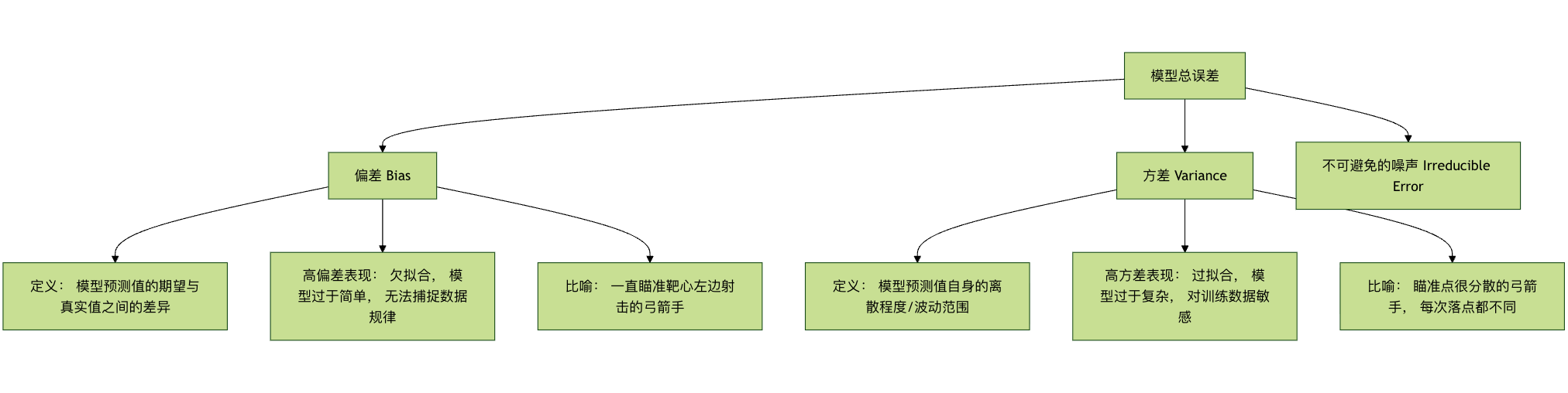
- Biasmeasures the model's ownsystematic error.High bias means the model is too simple, failing to even learn the basic patterns in the training data (underfitting).
- Variancemeasures the model's sensitivity torandom fluctuations in the training data.High variance means the model is too complex, treating noise in the training data as patterns to learn (overfitting).
Our goal is to find thebias-variance tradeoffoptimal point to minimize the total error. Regularization is a method that, byadding a bit of bias (making the model slightly simpler), significantly reduces variance, and thereby effectively improves the overall generalization performance of the model.
L1 and L2 Regularization
The most classic regularization method is to directly add a penalty term based on the model's weight parameters to the loss function. Depending on the calculation method of the penalty term, it is mainly divided into L1 and L2 regularization.
Changes in the Loss Function
Unregularized loss function (using Mean Squared Error, MSE, as an example):Loss = (1/n) * Σ(真实值 - 预测值)²
Loss function after adding the regularization term:Loss_正则化 = Loss + λ * Penalty(权重)
where:
λ(lambda) is theregularization strength coefficient,a hyperparameter greater than 0. It controls the strength of the penalty.λThe larger λ is, the heavier the penalty on model complexity, and the simpler the model becomes.Penalty(权重)is the penalty term. L1 and L2 have different definitions.
L1 Regularization (Lasso Regression)
- Penalty Term: The sum of the absolute values of all weight parameters in the model.
- Formula:
Penalty = Σ|w_i|, wherew_iis the i-th weight. - Loss Function:
Loss_L1 = Loss + λ * Σ|w_i|
Core Features and Effects:
- Feature Selection: L1 regularization tends to produce asparse weight matrix,, i.e., it will directly compress the weights of many unimportant features to00. This is equivalent to automatically completing feature selection, where the model only retains the most important features.
- Geometric Interpretation: Geometrically, its constraint region is a 'diamond' (a rhombus in two dimensions). The optimal solution point is more likely to touch a 'corner' of this diamond, and points at the corner mean some coordinates are 0.
Code Example:
Example
from sklearn.datasets import make_regression
from sklearn.model_selection import train_test_split
# Generate simulated data
X, y = make_regression(n_samples=100, n_features=10, noise=0.1, random_state=42)
X_train, X_test, y_train, y_test = train_test_split(X, y, test_size=0.2, random_state=42)
# Create L1 regularization model (Lasso), set regularization strength alpha (i.e., λ)
lasso_model = Lasso(alpha=0.1) # The larger alpha, the stronger the penalty, and more weights become 0
lasso_model.fit(X_train, y_train)
# View model coefficients (weights) to observe sparsity
print("Lasso model coefficients:")
for i, coef in enumerate(lasso_model.coef_):
print(f" Feature {i}: {coef:.4f}")
# Count the number of non-zero weights
non_zero_count = sum(lasso_model.coef_ != 0)
print(f"\nNumber of features with non-zero weights: {non_zero_count} / {X.shape)
Output:
Lasso 模型系数:
  特征 0: 16.6855
  特征 1: 54.0447
  特征 2: 5.0302
  特征 3: 63.5492
  特征 4: 93.4587
  特征 5: 70.5421
  特征 6: 86.9569
  特征 7: 10.2711
  特征 8: 3.0697
  特征 9: 70.7835

非零权重的特征数量: 10 / 10
L2 Regularization (Ridge Regression)
- Penalty Term: The sum of squares of all weight parameters in the model.
- Formula:
Penalty = Σ(w_i)² - Loss Function:
Loss_L2 = Loss + λ * Σ(w_i)²
Core Features and Effects:
- Weight Decay: L2 regularization tends to make all weight parametersapproach 0, but usually do not equal 0.It shrinks all weights uniformly, preventing any single weight from becoming too large.
- Improving Ill-Conditioned Problems: For data with multicollinearity (high correlation) among features, ordinary linear regression may be unstable. L2 regularization can effectively improve this problem and make the solution more stable.
- Geometric Interpretation: Geometrically, its constraint region is a 'circle' (a circle in two dimensions). The optimal solution point is more likely to touch the 'edge' of this circle rather than a sharp corner.
Code Example:
Example
# Create L2 regularization model (Ridge)
ridge_model = Ridge(alpha=1.0) # alpha is λ
ridge_model.fit(X_train, y_train)
# View model coefficients to observe weight decay
print("Ridge model coefficients:")
for i, coef in enumerate(ridge_model.coef_):
print(f" Feature {i}: {coef:.4f}")
# Compare the coefficient differences between Lasso and Ridge
print("\nCoefficient comparison (Lasso vs Ridge):")
print("Feature | Lasso coefficient | Ridge coefficient")
print("-" * 35)
for i in range(len(lasso_model.coef_)):
print(f"{i:4d} | {lasso_model.coef_[i]:11.4f} | {ridge_model.coef_[i]:11.4f}")
L1 vs L2 Comparison Summary
| Property | L1 Regularization (Lasso) | L2 Regularization (Ridge) |
|---|---|---|
| Penalty term | `Σ | w_i |
| Solution characteristics | Sparse solution, many weights are 0 | Dense solution, weights are close to 0 but not zero |
| Core function | Feature selection | Weight decay, Stable solution |
| Geometric shape | Diamond / polyhedron | Circle / sphere |
| Computation | More complex optimization (not differentiable everywhere) | Simple optimization (differentiable everywhere) |
| Applicable scenarios | Many features, and only a few are considered relevant | All features may contribute, or multicollinearity exists |
Elastic Net
Elastic Net is a compromise between L1 and L2 regularization, containing penalty terms of both.Loss_ElasticNet = Loss + λ1 * Σ|w_i| + λ2 * Σ(w_i)²
It combines L1's feature selection capability with L2's stability, making it suitable for cases with very high feature dimensions and correlations among features.
Example
elastic_model = ElasticNet(alpha=0.1, l1_ratio=0.5) # l1_ratio controls the mixing ratio of L1 and L2
elastic_model.fit(X_train, y_train)
Other Regularization Techniques
In addition to directly modifying the loss function, there are also methods that achieve regularization by changing the training process or model structure.
Dropout (for Neural Networks)
Dropout is an extremely effective regularization technique in neural networks. During thetraining process,it randomly causes a portion of neurons in the network to temporarily 'deactivate' (set their output to 0).
How It Works:
- In each training batch, with probability
p(e.g., 0.5), randomly drop a portion of neurons. - Forward propagation and backpropagation are performed only in the remaining neurons.
- During testing or prediction, all neurons are used, but the output of a neuron is multiplied by
(1-p)to keep the expected value consistent.
Core Idea: To prevent complex co-adaptation between neurons, forcing the network to learn morerobustanddispersedfeature representations. This is like a team: it cannot always rely on a few core members; everyone needs to be able to work independently, so that even if someone is absent, the team can still function normally.
Code example (using TensorFlow/Keras):
Example
from tensorflow.keras.models import Sequential
from tensorflow.keras.layers import Dense, Dropout
model = Sequential([
Dense(128, activation='relu', input_shape=(input_dim,)),
Dropout(0.5), # Add a Dropout layer after the previous layer, dropout rate 50%
Dense(64, activation='relu'),
Dropout(0.3), # dropout rate 30%
Dense(1, activation='sigmoid') # output layer
])
model.compile(optimizer='adam', loss='binary_crossentropy', metrics=['accuracy'])
Early Stopping
Early stopping is a simple and efficient regularization strategy. It does not modify the loss function, but insteadmonitors the model's performance on the validation set.。
Steps:
- Split the data into training and validation sets.
- Train the model on the training set, and periodically evaluate performance on the validation set (e.g., after each training epoch).
- Once it is found that the performance (e.g., loss) on the validation set has not improved over multiple consecutive epochsor has even started to decline,stop training immediately.
Core idea:Stop training at the moment just before the model begins to overfit the training data (i.e., when the validation error starts to rise), thereby obtaining the model weights with the best generalization ability.
Example
# Define the early stopping callback function
# monitor: the metric to monitor, e.g., 'val_loss'
# patience: number of epochs to tolerate; stop if validation performance does not improve within this many epochs
# restore_best_weights: whether to restore the weights from the epoch with the best monitored metric
early_stopping = EarlyStopping(
monitor='val_loss',
patience=10,
restore_best_weights=True
)
# Use in model.fit
history = model.fit(
X_train, y_train,
validation_data=(X_val, y_val),
epochs=100,
callbacks=[early_stopping] # Pass the callback list
)
Practice Exercise: Comprehensive Comparison of Regularization Effects
Let's use a complete example to compare the effects of different regularization methods on a regression task.
Example
import matplotlib.pyplot as plt
from sklearn.linear_model import LinearRegression, Lasso, Ridge, ElasticNet
from sklearn.preprocessing import PolynomialFeatures
from sklearn.pipeline import make_pipeline
from sklearn.metrics import mean_squared_error
# 1. Generate nonlinear data with noise
np.random.seed(42)
X = np.linspace(-3, 3, 100).reshape(-1, 1)
y_true = 0.5 * X.ravel()**2 + X.ravel() # True quadratic relationship
y = y_true + np.random.randn(100) * 0.8 # Add noise
# 2. Create models of different complexity (using polynomial features)
degree = 10 # Use a 10th-degree polynomial, which is prone to overfitting
models = {
'No regularization': make_pipeline(PolynomialFeatures(degree), LinearRegression()),
'L1 (Lasso)': make_pipeline(PolynomialFeatures(degree), Lasso(alpha=0.01, max_iter=10000)),
'L2 (Ridge)': make_pipeline(PolynomialFeatures(degree), Ridge(alpha=0.1)),
'ElasticNet': make_pipeline(PolynomialFeatures(degree), ElasticNet(alpha=0.01, l1_ratio=0.5))
}
# 3. Train and predict
X_plot = np.linspace(-3.5, 3.5, 200).reshape(-1, 1)
plt.figure(figsize=(12, 8))
plt.scatter(X, y, s=20, alpha=0.6, label='Training data (with noise)')
plt.plot(X, y_true, 'k-', linewidth=3, label='True function')
for name, model in models.items():
model.fit(X, y)
y_plot = model.predict(X_plot)
mse = mean_squared_error(y, model.predict(X))
plt.plot(X_plot, y_plot, '--', linewidth=2, label=f'{name} (MSE: {mse:.3f})')
plt.xlabel('X')
plt.ylabel('y')
plt.title('Comparison of different regularization methods in suppressing overfitting (10th-degree polynomial)')
plt.legend(loc='best')
plt.grid(True, alpha=0.3)
plt.show()
Practice tasks:
- Run the above code and observe how the unregularized model fluctuates wildly to fit noise (overfitting), while the regularized model curves are smoother and closer to the true function.
- Try adjusting
degree(the polynomial degree) and each model'salpha(regularization strength) parameters, and observe their impact on the model fitting results. - (Advanced) Split the data into training and test sets, compute the MSE of each model on the test set, and verify the improvement in generalization from regularization.
Summary and Engineering Recommendations
Regularization is an essential tool in a machine learning engineer's toolbox. To apply it effectively, keep the following points in mind:
- Understand the nature of the problem:First, use learning curves, validation set performance, etc., to determine whether the model faces an overfitting (high variance) problem.
- Start simple:Usually, you can first tryL2 regularization,because it is stable and easy to tune. If the feature dimensionality is extremely high and feature selection is needed, then considerL1orelastic net.。
- Tuning is key:The regularization strength
λ(oralpha) is a crucial hyperparameter. It must becross-validationto carefully select. - Use in combination:In practice, regularization techniques are often used in combination. For example, when training deep neural networks,Dropout + L2 weight decay + early stoppingis an extremely common combination.
- Domain adaptation:For computer vision tasks, Dropout and Batch Normalization (which also has a certain regularization effect) are very effective. For sequence models (such as RNN, Transformer), Dropout and weight decay are commonly used.
The ultimate goal of regularization is to guide the model from "rote memorization" of training data toward "deep understanding" of the universal patterns behind the data, so as to make more reliable predictions in the real world. Master it, and you hold the key to improving model generalization.
Other extensions