Reinforcement Learning Exploration vs Exploitation
In the world of reinforcement learning, the agent is like an explorer who constantly learns and grows in an unknown environment. It faces a core contradiction that runs throughout: should itexplore (Exploration)unknown territory and look for new paths that may bring higher rewards, or should itexploit (Exploitation)the known best strategy to steadily obtain the currently known maximum reward? This "exploration-exploitation trade-off" is one of the most fundamental and critical challenges in reinforcement learning algorithm design. Understanding and handling this contradiction well is the necessary path for an agent to grow from a novice to a master.
What are exploration and exploitation?
Let us first understand these two core concepts through an analogy from daily life.
Imagine that every day at noon you have to choose a restaurant for lunch.
- Exploitation: You choose to go to theknown restaurant you like the most. You know the food there suits your taste, the prices are reasonable, and the service quality is stable. Choosing exploitation means you make decisions based onthe best currently known information, with the goal ofmaximizing the certain immediate gains. In reinforcement learning, this corresponds to the agent choosing the action with the highest current estimate (such as the Q-value).
- Exploration: You decide totry a new restaurant you have never visited. This new restaurant may be awful and make you regret it deeply, but it may also be unexpectedly delicious and become your new favorite. Choosing exploration means youtake action in order to obtain more information about the environment, with the goal ofoptimizing long-term future rewards. In reinforcement learning, this corresponds to the agent randomly selecting actions, or selecting actions that are not currently optimal, so as to update its understanding of the environmental model.
The goal of a reinforcement learning agent is not to win a single lunch, but toobtain the greatest long-term satisfaction (cumulative reward) across countless lunch choices.If you only exploit and never explore, you may never discover that better new restaurant, and long-term rewards cannot reach the optimum. If you only explore and never exploit, you may waste a lot of time and money on bad restaurants and fail to enjoy the best known choice.
Why is a trade-off needed?
The reason exploration and exploitation need a trade-off is rooted in theuncertaintyof the environment and theincompleteness of the agent's knowledge.。
- Limited information: The agent initially knows nothing about the environment. It must collect data through exploration to build a cognitive model of the world (states, actions, rewards, transition probabilities).
- Opportunity cost: Exploring unknown actions may yield lower immediate rewards (or even punishment), which is equivalent to paying a cost for information. Excessive exploration will sacrifice a large amount of short-term reward that could otherwise have been obtained.
- Dynamic nature of the optimal solution: In non-stationary environments, the optimal policy may change over time. Even if the agent has found the current optimal policy, it still needs to continue exploring to a certain degree to adapt to environmental changes and prevent the policy from becoming outdated.
Therefore, an excellent reinforcement learning algorithm must find a dynamic balance between "using existing knowledge to obtain rewards" and "exploring the unknown to improve knowledge."
Common exploration strategies
How can exploration mechanisms be integrated into an algorithm? Here are several classic methods:
ε-Greedy Strategy (ε-Greedy)
This is the simplest and most commonly used exploration strategy. The agent, most of the time (with probability1-ε) chooses the action it currently believes to be optimal (exploitation), but with a small probabilityε(for example, 5%) chooses an action completely at random (exploration).
Example
def epsilon_greedy(q_values, epsilon=0.1):
"""
Implementing the ε-Greedy Strategy
Args:
q_values: an array representing the Q-value estimate of each action in the current state.
epsilon: the exploration probability, between 0 and 1.
Returns:
selected_action: the index of the action selected according to the strategy.
"""
n_actions = len(q_values)
# Explore with probability epsilon (random selection)
if np.random.random() < epsilon:
selected_action = np.random.randint(n_actions)
# Exploit with probability 1-epsilon (choose the action with the largest Q-value)
else:
# If multiple actions have the same Q-value, choose one at random
selected_action = np.random.choice(np.where(q_values == np.max(q_values))[0])
return selected_action
# Example: suppose in a certain state, the Q-value estimates of the three actions are [1.5, 2.8, 2.3]
state_q_values = [1.5, 2.8, 2.3]
for i in range(10):
action = epsilon_greedy(state_q_values, epsilon=0.2)
print(f"Selection {i+1}: Action {action} (Q-value: {state_q_values[action]:.1f})")
Advantages: Simple and easy to understand, easy to implement.Disadvantages: Exploration is completely random and does not use any existing information (for example, although an action is not optimal, its Q-value is close to the optimal one; its probability of being explored is the same as that of a bad action with a very low Q-value).
Upper Confidence Bound Algorithm (Upper Confidence Bound, UCB)
UCB is a "smarter" exploration strategy. Its core idea is to add an "uncertainty bonus" to the estimate of each action. The fewer times an action has been tried, the greater its uncertainty, and the higher this bonus term is, thereby encouraging the agent to try it.
The action selection formula is usually: \[ a_t = \arg\max_a \left[ Q(a) + c \sqrt{\frac{\ln t}{N_t(a)}} \right] \]
where:
Q(a)is the action'sacurrent average reward estimate (exploitation term).N_t(a)is, up to timet, the number of times actionahas been selected.cis a balance parameter that controls the strength of exploration.ln tis the logarithm of the total time step.- The square-root term is the "uncertainty bonus" or "exploration bonus." The fewer times an action is selected (
N_t(a)is small), the larger this term becomes.
Example
import math
class UCB:
def __init__(self, n_actions, c=2):
self.n_actions = n_actions
self.c = c # Exploration parameter
self.Q = np.zeros(n_actions) # Action value estimates
self.N = np.zeros(n_actions) # Action selection counts
self.total_steps = 0
def select_action(self):
self.total_steps += 1
# Ensure each action is selected at least once
if np.any(self.N == 0):
action = np.random.choice(np.where(self.N == 0)[0])
else:
# Calculate the UCB value of each action: Q(a) + c * sqrt(ln(t) / N(a))
ucb_values = self.Q + self.c * np.sqrt(np.log(self.total_steps) / self.N)
action = np.argmax(ucb_values)
return action
def update(self, action, reward):
"""Update the value estimate of the action"""
self.N[action] += 1
# Incrementally update the Q-value: NewEstimate = OldEstimate + (1/N) * (Target - OldEstimate)
self.Q[action] += (reward - self.Q[action]) / self.N[action]
# Simulate a multi-armed bandit problem, where each arm has a different true reward probability
true_means = [0.1, 0.5, 0.9] # True average rewards of the three arms
n_actions = len(true_means)
bandit = UCB(n_actions, c=2)
total_reward = 0
for step in range(1000):
action = bandit.select_action()
# Simulate pulling a bandit arm, obtaining reward 1 with a certain probability, otherwise 0
reward = 1 if np.random.random() < true_means[action] else 0
bandit.update(action, reward)
total_reward += reward
print(f"Total reward obtained by the UCB strategy after 1000 steps: {total_reward}")
print(f"Number of times each action was selected: {bandit.N}")
print(f"Q-value estimates of each action: {bandit.Q}")
Advantages: Exploration is more purposeful; it preferentially explores actions with high uncertainty (few attempts), and can converge to the optimal action faster.Disadvantages: It needs to maintain the number of times each action is selected, and it may not be applicable when the action space is continuous or very large.
Thompson Sampling
This is a probabilistic method based on Bayesian ideas. For the reward distribution of each action (e.g., the parameter of a Bernoulli distributionθ_a), the agent maintains a prior distribution (such as a Beta distribution). At each step, from the posterior distribution of each action, itsamplesa possible reward parameterθ_a, and then executes the action with the largest sampled value. After receiving the actual reward, it updates the posterior distribution of that action according to the result.
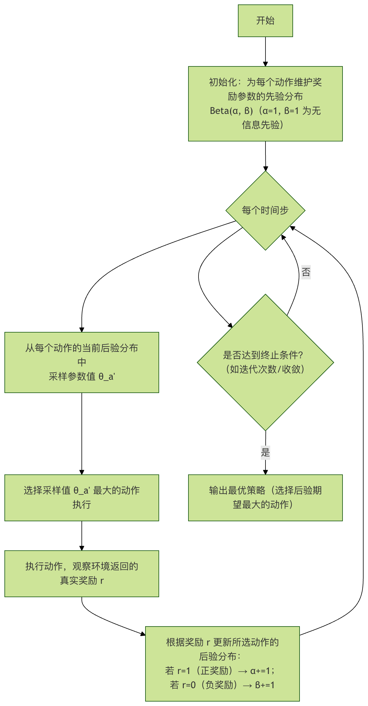
Procedure explanation:
- Initialization: For each action
aassume the probability of obtaining a rewardθ_afollows a Beta(α=1, β=1) distribution, which is a uniform prior. - Sampling: At each step, from each action's
acurrent Beta(α_a, β_a) distribution, independently sample a valueθ_a'。 - Selection: Execute the action with the sampled value
θ_a'that is the largest. - Update: If a reward is obtained
r=1, then the action'sαincrement by 1; ifr=0, then theβincrement by 1. This is equivalent to updating the Bayesian posterior distribution with observed data.
Advantages: Naturally balances exploration and exploitation, has good theoretical properties, and often performs very well in practice.Disadvantages: It requires assuming the form of the reward distribution, and the computation may be more complex than ε-greedy.
Dynamic balance between exploration and exploitation
In practical applications, exploration strategies are often not static but are dynamically adjusted as the agent's learning process progresses.
- Heavy exploration in the early stage: At the beginning of training, the agent knows nothing about the environment, so a higher exploration rate should be set (such as a larger
εorc), to collect data extensively. - Heavy exploitation in the later stage: As learning proceeds, the agent's understanding of the environment becomes more accurate, and the exploration rate should be gradually reduced (for example, let
εdecay over time), shifting the focus to exploiting the excellent strategies already learned, in order to steadily obtain high returns.
This dynamic adjustment process simulates the human learning process of "from extensive trying to continuous improvement."
Hands-on Exercise: Comparing Different Strategies
Let us design a simple experiment to compare the performance of ε-greedy and UCB strategies on the classic "multi-armed bandit" problem.
Task:
- Create a bandit with 5 arms, where the true reward probabilities of each arm are respectively
[0.1, 0.2, 0.8, 0.5, 0.3]。 - Implement the ε-greedy (ε=0.1) and UCB (c=2) strategies respectively.
- Run each strategy for 2000 steps, recording the immediate reward and cumulative reward at each step.
- Plot the curve of cumulative reward over time steps, and observe which strategy can obtain higher total reward faster and more stably.
Think:
- Try adjusting the ε and c parameters and observe what impact they have on the results?
- If the gap between the optimal arm (probability 0.8) and the suboptimal arm (probability 0.5) becomes smaller, how will the performance of the strategies change?
- In more complex reinforcement learning environments (such as
Gym), how can these exploration strategies be combined with Q-Learning, DQN, and other algorithms?