Logistic Regression
Logistic Regression is a statistical learning method widely used for classification problems. Despite having "regression" in its name, it is actually an algorithm for binary or multi-class classification problems.
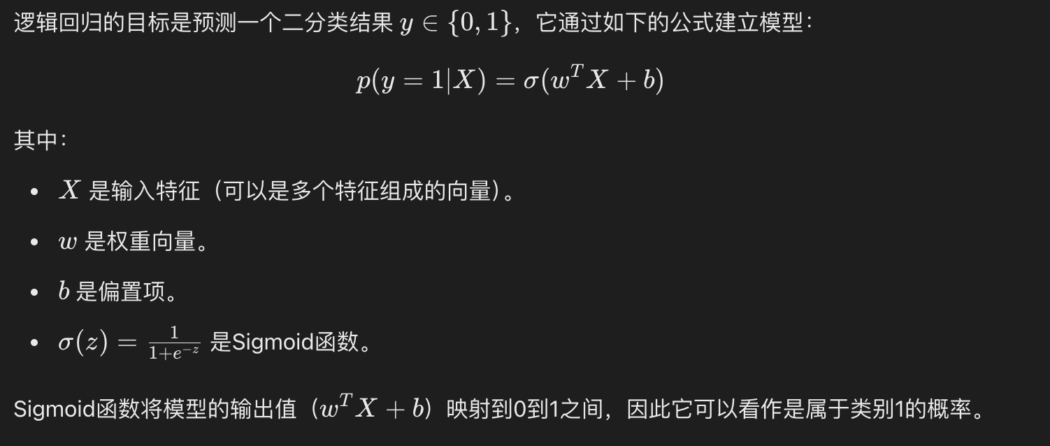
Logistic regression uses a logistic function (also called the Sigmoid function) to map the output of linear regression to between 0 and 1, thereby predicting the probability of a certain event occurring.
Logistic regression is widely used in various classification problems, such as:
- Spam detection (spam / not spam)
- Disease prediction (disease / no disease)
- Customer churn prediction (churn / no churn)
Logistic Regression Model
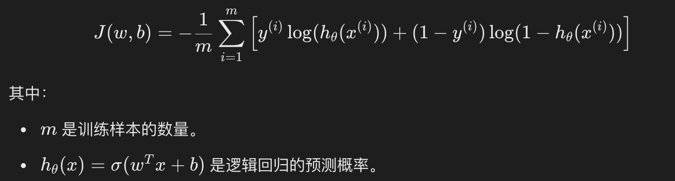
Loss Function
The loss function of logistic regression is the Log Loss, which is of the following form:
Solving with Gradient Descent
Like linear regression, logistic regression usually also uses gradient descent to optimize the loss function and solve for parameters w and b. The gradient update rules for logistic regression are as follows:
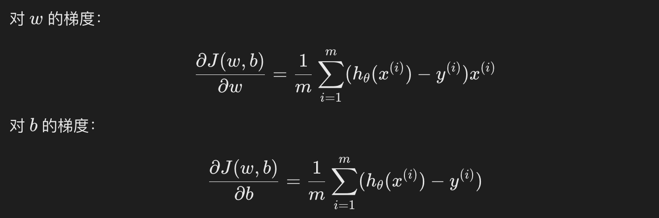
By continuously updating w and b until the loss function converges.
Implementing Logistic Regression with Python
Next, we will use Python and the Scikit-learn library to implement a simple logistic regression model.
1. Import necessary libraries
Example
import matplotlib.pyplot as plt
from sklearn.datasets import load_iris
from sklearn.model_selection import train_test_split
from sklearn.linear_model import LogisticRegression
from sklearn.metrics import accuracy_score, confusion_matrix, classification_report
2. Load dataset
We will use the Iris dataset that comes with Scikit-learn. The Iris dataset contains 150 samples, each with 4 features, and the goal is to classify the samples into 3 classes. To simplify the problem, we only use the first two features and convert the problem into a binary classification problem.
Example
iris = load_iris()
X = iris.data[:, :2] # Only use first two features
y = (iris.target != 0) * 1 # Convert target to binary classification problem
# Split training and test sets
X_train, X_test, y_train, y_test = train_test_split(X, y, test_size=0.3, random_state=42)
3. Train logistic regression model
Example
model = LogisticRegression()
# Train model
model.fit(X_train, y_train)
4. Model evaluation
Example
import matplotlib.pyplot as plt
from sklearn.datasets import load_iris
from sklearn.model_selection import train_test_split
from sklearn.linear_model import LogisticRegression
from sklearn.metrics import accuracy_score, confusion_matrix, classification_report
# Load dataset
iris = load_iris()
X = iris.data[:, :2] # Only use first two features
y = (iris.target != 0) * 1 # Convert target to binary classification problem
# Split training and test sets
X_train, X_test, y_train, y_test = train_test_split(X, y, test_size=0.3, random_state=42)
# Create logistic regression model
model = LogisticRegression()
# Train model
model.fit(X_train, y_train)
# Predict test set
y_pred = model.predict(X_test)
# Calculate accuracy
accuracy = accuracy_score(y_test, y_pred)
print(f"Model accuracy: {accuracy:.2f}")
# Confusion matrix
conf_matrix = confusion_matrix(y_test, y_pred)
print("Confusion matrix:")
print(conf_matrix)
# Classification report
class_report = classification_report(y_test, y_pred)
print("Classification report:")
print(class_report)
The output is:
模型准确率: 1.00
混淆矩阵:
[[19  0]
 [ 0 26]]
分类报告:
              precision    recall  f1-score   support

           0       1.00      1.00      1.00        19
           1       1.00      1.00      1.00        26

    accuracy                           1.00        45
   macro avg       1.00      1.00      1.00        45
weighted avg       1.00      1.00      1.00        45
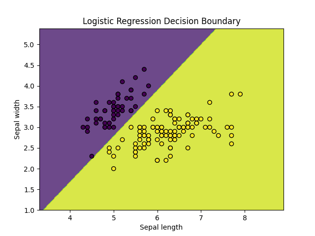
5. Visualize decision boundary
Example
import matplotlib.pyplot as plt
from sklearn.datasets import load_iris
from sklearn.model_selection import train_test_split
from sklearn.linear_model import LogisticRegression
from sklearn.metrics import accuracy_score, confusion_matrix, classification_report
# Load dataset
iris = load_iris()
X = iris.data[:, :2] # Only use first two features
y = (iris.target != 0) * 1 # Convert target to binary classification problem
# Split training and test sets
X_train, X_test, y_train, y_test = train_test_split(X, y, test_size=0.3, random_state=42)
# Create logistic regression model
model = LogisticRegression()
# Train model
model.fit(X_train, y_train)
# Predict test set
y_pred = model.predict(X_test)
# Visualize decision boundary
x_min, x_max = X[:, 0].min() - 1, X[:, 0].max() + 1
y_min, y_max = X[:, 1].min() - 1, X[:, 1].max() + 1
xx, yy = np.meshgrid(np.arange(x_min, x_max, 0.01),
np.arange(y_min, y_max, 0.01))
Z = model.predict(np.c_[xx.ravel(), yy.ravel()])
Z = Z.reshape(xx.shape)
plt.contourf(xx, yy, Z, alpha=0.8)
plt.scatter(X[:, 0], X[:, 1], c=y, edgecolors='k', marker='o')
plt.xlabel('Sepal length')
plt.ylabel('Sepal width')
plt.title('Logistic Regression Decision Boundary')
plt.show()
Displayed as follows:
Summary
- Logistic regression uses the Sigmoid function to convert the output of linear regression into probability values, and is used to solve binary classification problems.
- The training process of logistic regression optimizes model parameters by minimizing the log loss function.
- Gradient descent is a commonly used optimization method to update model parameters.and。
- In Python, the
scikit-learnlibrary provides a simple and easy-to-use interface for implementing logistic regression, and makes it easy to train, evaluate, and visualize models.