Unsupervised Learning - Dimensionality Reduction
Imagine you are a photographer organizing a library containing millions of high-resolution photos. Each photo is composed of millions of pixels (features). If you want to quickly find all photos of sunsets by the sea, directly comparing every pixel of each photo is almost impossible, because the data is too large and too "fat".
In machine learning, we often face a similar dilemma: datasets have hundreds or thousands of features (dimensions). This not only leads to extremely slow computation (the curse of dimensionality), but may also, because many features are redundant or irrelevant, interfere with our ability to find the true patterns in the data.
Dimensionality Reduction is a core technique in unsupervised learning. It acts like a data fitness coach, helping us slim down high-dimensional data into a lower-dimensional space while preserving the most important information as much as possible. Today, let's learn dimensionality reduction in a simple and thorough way.Basic Concepts of Dimensionality Reduction
Basic Concepts of Dimensionality Reduction
What is Dimensionality Reduction?
dimensionality reduction is the process of reducing the number of features in a dataset.It uses a mathematical transformation to map data points from the original high-dimensional space into a new space with lower dimensionality.Why perform dimensionality reduction?
Why Dimensionality Reduction?
Visualization
- : Humans can intuitively understand at most three-dimensional space. By reducing dimensions to 2D or 3D, we can plot high-dimensional data and intuitively observe its structure, groupings, and outliers.Improved efficiency
- : Fewer data dimensions mean less storage space, faster training speed, and lower computational cost.Removing noise and redundancy
- : Many algorithms (especially distance-computation algorithms such as KNN) suffer performance degradation in high-dimensional space due to irrelevant or duplicate features. Dimensionality reduction can distill the essence of the data.Mitigating the curse of dimensionality
- : In high-dimensional space, data becomes extremely sparse, making it difficult for many machine learning models to find effective patterns.Core Idea: Information Preservation
Core Idea: Information Preservation
How to reduce dimensions while maximizing the preservation of valuable information in the original data (such as variance and data structure)?Different dimensionality reduction algorithms have different answers to this.Detailed Explanation of Mainstream Dimensionality Reduction Algorithms
Detailed Explanation of Mainstream Dimensionality Reduction Algorithms
Linear dimensionality reductionNonlinear dimensionality reductionandLinear Dimensionality Reduction: Principal Component Analysis。
Linear Dimensionality Reduction: Principal Component Analysis
How PCA works (four steps):Centering
: Subtract the mean of each feature so that the center of the data distribution moves to the origin of the coordinate system.
- Compute the covariance matrix: This matrix describes the correlations between the various features of the data.
- Eigenvalue decomposition: Compute the eigenvalues and eigenvectors of the covariance matrix.
- The eigenvectorsindicate the directions of the new coordinate axes (principal components),while the eigenvaluesrepresent the variance of the data along that direction. The larger the eigenvalue, the more information that direction contains.Selecting principal components: Sort the eigenvalues from largest to smallest, and select the top
- eigenvectors corresponding to the largest eigenvalues to form a projection matrix.Data transformation
k: Multiply the original data by this projection matrix to obtain data reduced to - dimensions.Example
k# Import necessary libraries
Example
import numpy as np
import matplotlib.pyplot as plt
from sklearn.decomposition import PCA
from sklearn.datasets import load_iris
# macOS first
plt.rcParams['font.sans-serif'] = [
# Linux first
'SimHei', 'Microsoft YaHei',
# Fix the issue where negative signs display as squares
'PingFang SC', 'Heiti TC',
# -------------------------- Set Chinese font end --------------------------
'WenQuanYi Micro Hei', 'DejaVu Sans'
]
# 1. Load the classic Iris dataset (4 features)
plt.rcParams['axes.unicode_minus'] = False
# Original data: 150 samples, 4 features
# Labels, used for coloring in visualization
iris = load_iris()
X = iris.data "Original data shape: {X.shape}"
y = iris.target # Output: (150, 4)
print(f# 2. Create a PCA model, specify reducing to 2 dimensions) # 3. Fit the model (compute principal components) and transform the data
"Data shape after dimensionality reduction: {X_pca.shape}"
pca = PCA(n_components=2)
# Output: (150, 2)
X_pca = pca.fit_transform(X)
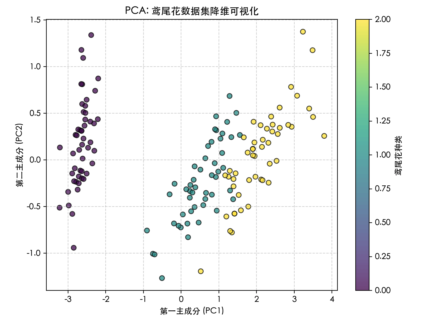
print(f"Variance ratio explained by each principal component: {pca.explained_variance_ratio_}") # Output might be similar to: [0.9246, 0.0530] indicating the first principal component retains 92.5% of the information, and the second retains 5.3%
print(f# 4. Visualize the dimensionality reduction result)
'First Principal Component (PC1)'
'Second Principal Component (PC2)'
plt.figure(figsize=(8, 6))
scatter = plt.scatter(X_pca[:, 0], X_pca[:, 1], c=y, edgecolor='k', alpha=0.7)
plt.xlabel('PCA: Visualization of Iris Dataset Dimensionality Reduction')
plt.ylabel('Iris species')
plt.title(Code explanation)
plt.colorbar(scatter, label=: Initialize the model,)
plt.grid(True, linestyle='--', alpha=0.5)
plt.show()
the parameter specifies the number of principal components to retain (i.e., the dimensionality after reduction).:
PCA(n_components=2): This is a combination method; first it computes the mean and principal component directions of the data (n_components), then immediately transforms the data into the new space (fit_transform(X): This is a very important attribute of PCA; it tells us how much variance (information) of the original data each new feature (principal component) retains. This helps us decide how many principal components are appropriate to choose.fitPros and Cons of PCAtransform)。explained_variance_ratio_Advantages
: Computationally efficient, clear principles, and can effectively remove linear correlations.
- Disadvantages: It is a linear method and assumes that the principal components of the data are linear. For nonlinear manifold data such as the "Swiss roll", PCA does not perform well.
- Nonlinear Dimensionality Reduction: t-SNEWhen data has complex nonlinear structures, we need nonlinear dimensionality reduction methods.
Nonlinear Dimensionality Reduction: t-SNE
Core Idea of t-SNEt-SNE focuses onpreserving the local structure of the data.
It tries to make points that are "similar" (close in distance) in the high-dimensional space also "similar" in the low-dimensional mapping; while points that are "not similar" in high-dimensional space become far apart in low-dimensional space.
Example# Import necessary libraries# Generate Swiss roll data
Example
import numpy as np
import matplotlib.pyplot as plt
from sklearn.decomposition import PCA
from sklearn.manifold import TSNE
from sklearn.datasets import make_swiss_roll # macOS first
# Linux first
plt.rcParams['font.sans-serif'] = [
# Fix the issue where negative signs display as squares
'SimHei', 'Microsoft YaHei',
# -------------------------- Set Chinese font end --------------------------
'PingFang SC', 'Heiti TC',
# 1. Generate a nonlinear dataset: Swiss roll
'WenQuanYi Micro Hei', 'DejaVu Sans'
]
"Swiss roll data shape: {X_swiss.shape}"
plt.rcParams['axes.unicode_minus'] = False
# 2. Use PCA (linear method) to attempt dimensionality reduction
# 3. Use t-SNE (nonlinear method) for dimensionality reduction
X_swiss, color = make_swiss_roll(n_samples=1000, noise=0.1)
print(f# perplexity is a key parameter of t-SNE, usually between 5 and 50, representing a balanced focus on local/global structure) # (1000, 3)
# 4. Compare visualizations
pca = PCA(n_components=2)
X_swiss_pca = pca.fit_transform(X_swiss)
# PCA result
'PCA Dimensionality Reduction Result'
tsne = TSNE(n_components=2, perplexity=30, random_state=42)
X_swiss_tsne = tsne.fit_transform(X_swiss)
# t-SNE result
fig, axes = plt.subplots(1, 2, figsize=(15, 6))
't-SNE Dimensionality Reduction Result (perplexity=30)'
axes[0].scatter(X_swiss_pca[:, 0], X_swiss_pca[:, 1], c=color, cmap='viridis')
axes[0].set_title('Swiss roll "height"')
axes[0].set_xlabel('PC1')
axes[0].set_ylabel('PC2')
How to Choose Dimensionality Reduction Methods and Key Parameters
sc = axes[1].scatter(X_swiss_tsne[:, 0], X_swiss_tsne[:, 1], c=color, cmap='viridis')
axes[1].set_title(Algorithm Selection Flowchart)
axes[1].set_xlabel('t-SNE 1')
axes[1].set_ylabel('t-SNE 2')
plt.colorbar(sc, ax=axes[1], label=Key Parameter Guide)
plt.tight_layout()
plt.show()
Code Explanation:
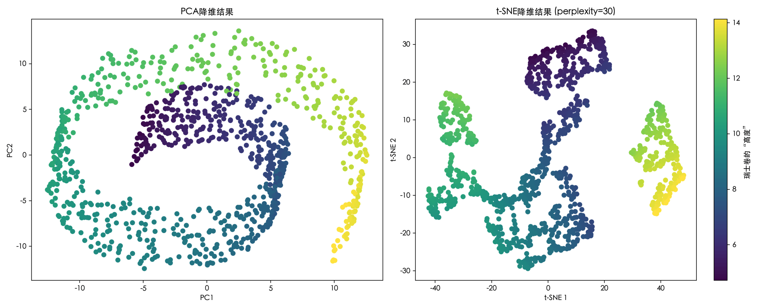
perplexityParameter: can be understood as how many neighbors to consider for each point. Smaller values focus more on local structure, larger values focus more on global structure. It is the most important parameter to tune in t-SNE.random_state: ensures results are reproducible, because the t-SNE optimization process is stochastic.- From the visualization results, it is clear that PCA "flattens" the Swiss roll, losing its nonlinear curling structure; while t-SNE better unfolds this roll on a 2D plane, preserving the local adjacency relationships of the data.
Advantages and Disadvantages of t-SNE
Advantages: Excellent visualization effect on complex nonlinear data, clearly showing cluster structures.
Disadvantages:
- Slow computation speed, not suitable for large datasets.
- Results haverandomness, each run may be slightly different.
- Sensitive to hyperparameters,
perplexityNeed tuning. - Mainlyused for visualization(2D/3D), the reduced-dimension features are usually not used for subsequent machine learning tasks, because the meaning of distances in the low-dimensional space has changed.
How to Choose Dimensionality Reduction Methods and Key Parameters
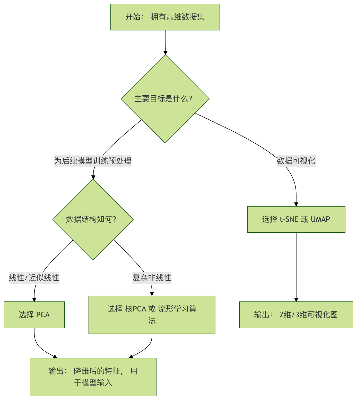
Algorithm Selection Flowchart
Key Parameter Guide
PCA: n_components
- Can be set to an integer (e.g., 2) to specify a specific dimension.
- Can be set to
0 < n < 1a decimal (e.g., 0.95), meaning retaincumulative explained variance ratioreaching the threshold with the minimum number of principal components.
Example
pca = PCA(n_components=0.95)
pca.fit(X)
print(f"To retain 95% variance, {pca.n_components_} principal components are needed")
t-SNE: perplexity
- Typical values are between 5 and 50.
- For small datasets (<100 samples), smaller values are recommended.
- The optimal value is usually close to the number of "neighbors" for each point in the data. It needs to be chosen by experimenting and observing the visualization results.
Practical Exercises and Summary
Hands-on Exercise: Applying Dimensionality Reduction on the MNIST Handwritten Digit Dataset
Example
from sklearn.preprocessing import StandardScaler
# 1. Load MNIST dataset (take only a subset of samples to speed up)
mnist = fetch_openml('mnist_784', version=1, as_frame=False)
X_mnist, y_mnist = mnist.data[:3000] / 255.0, mnist.target[:3000] # Normalize, take the first 3000 samples
print(f"MNIST data shape: {X_mnist.shape}") # (3000, 784) -> 784 dimensions!
# 2. First use PCA to quickly reduce to 50 dimensions, removing a lot of noise
pca = PCA(n_components=50)
X_mnist_pca = pca.fit_transform(X_mnist)
print(f"Shape after PCA: {X_mnist_pca.shape}")
# 3. Then use t-SNE to reduce the 50-dimensional data to 2 dimensions for visualization
tsne = TSNE(n_components=2, perplexity=40, n_iter=300, random_state=42)
X_mnist_tsne = tsne.fit_transform(X_mnist_pca)
# 4. Visualization
plt.figure(figsize=(10, 8))
scatter = plt.scatter(X_mnist_tsne[:, 0], X_mnist_tsne[:, 1],
c=y_mnist.astype(int), cmap='tab10', alpha=0.6, s=5)
plt.colorbar(scatter, ticks=range(10), label='Handwritten digits')
plt.title('t-SNE visualization of the MNIST handwritten digit dataset after PCA preprocessing')
plt.xlabel('t-SNE 1')
plt.ylabel('t-SNE 2')
plt.grid(True, linestyle='--', alpha=0.3)
plt.show()
Exercise Goal: Observe whether different digits (0-9) form clear clusters on the 2D plane. Try modifyingperplexityparameters (e.g., change to 10 or 50) and see how the visualization changes.
Summary and Key Points
The essence of dimensionality reduction: It is information compression and extraction, not simply discarding data. The goal isto express as much original information as possible with fewer dimensions.。
PCA (the king of linear methods): Finds the most important linear directions of data by maximizing variance. Efficient and stable, suitable for preprocessing and removing linear correlations.
t-SNE (a powerful tool for visualization): Reveals nonlinear structures by maintaining local similarities between data points. The effect is stunning, but it is slow and results are random, mainly used for exploratory data analysis.
Workflow:
- Clarify the goal: Is it for visualization, or to provide more refined features for downstream models?
- Data exploration: First visualize part of the data to get a preliminary sense of its linearity/nonlinearity.
- Method experimentation: Choose algorithms based on the goal and data structure, and adjust key parameters.
- Evaluate results: Evaluate the dimensionality reduction effect through visualization, information retention rate, or downstream task performance.
Dimensionality reduction is a key to unlocking the black box of high-dimensional data.
By mastering PCA and t-SNE, you can not only get an overview of the global structure when facing complex data, but also prepare streamlined features for subsequent machine learning models, greatly improving the efficiency and depth of data analysis.
Other Extensions