Data Visualization
Before starting to build a complex machine learning model, the first thing we need to do is not to choose an algorithm, but tounderstand the data.。
If we compare machine learning to cooking, then data is the ingredient.
An excellent chef must understand the characteristics of the ingredients — whether they are fresh or spoiled, whether they are sweet or sour, whether they are suitable for stewing or stir-frying.
Data visualization is ourmagnifying glassandand taste bud。
Data visualization uses visual elements such as charts and graphs to transform dull numbers into intuitive images, helping us to:
- Discover patterns and trends in the data(For example: Does sales revenue vary with the seasons?)
- Identify outliers and erroneous data(For example: a record with an age of 300 years)
- Understand relationships between features (variables)(For example: Are house area and price positively correlated?)
- Validate assumptions, and provide a basis for subsequent feature engineering and model selection.
This article will use the most popular data science libraries in Pythonpandasand visualization librariesmatplotlib、seaborn, to help you master the core skills of data visualization.
Preparation: Environment and Data
Before we start drawing charts, we need to prepare the "canvas" and "paint".
Install the necessary libraries
If you are using Anaconda, these libraries are usually pre-installed. Otherwise, you can install them with the following command:
pip install pandas matplotlib seaborn
Import libraries and load data
We will use a classic public dataset: the Titanic passenger dataset. It contains information about passenger survival, class, age, gender, and so on.
Example
import pandas as pd
import matplotlib.pyplot as plt
import seaborn as sns
# Set the chart style to make it look better
sns.set_style("whitegrid")
# -------------------------- Set Chinese font start --------------------------
plt.rcParams['font.sans-serif'] = [
# Windows first
'SimHei', 'Microsoft YaHei',
# macOS first
'PingFang SC', 'Heiti TC',
# Linux first
'WenQuanYi Micro Hei', 'DejaVu Sans'
]
# Fix the issue where the minus sign displays as a square
plt.rcParams['axes.unicode_minus'] = False
# -------------------------- Set Chinese font end --------------------------
# Load data
# Here we load directly from seaborn's built-in dataset
df = sns.load_dataset('titanic')
# View the first few rows and basic information of the data
print("Data shape (rows, columns):", df.shape)
print("\n"First 5 rows of data:")
print(df.head())
print("\n"Basic data information (types, non-null counts, etc.):")
print(df.info())
# Load data
# Here we load directly from seaborn's built-in dataset
df = sns.load_dataset('titanic')
# View the first few rows and basic information of the data
print("Data shape (rows, columns):", df.shape)
print("\n"First 5 rows of data:")
print(df.head())
print("\n"Basic data information (types, non-null counts, etc.):")
print(df.info())
Running the code above, you will see that the data has 891 rows (passengers) and 15 columns (features).df.head()This gives you an initial impression of what the data looks like.
Univariate Analysis: Understanding the Distribution of a Single Feature
Univariate analysis focuses onthe distribution of a singlefeature (variable). This is the most basic analysis.
1. Numerical Features: Histograms and Box Plots
For features such asage(age),fare(fare) and other continuous numerical features, we often usehistogramsandand box plots.。
Histogramdisplays the frequency distribution of data in different intervals ("bins").
Example
import pandas as pd
import matplotlib.pyplot as plt
import seaborn as sns
# Set the chart style to make it look better
sns.set_style("whitegrid")
# -------------------------- Set Chinese font start --------------------------
plt.rcParams['font.sans-serif'] = [
# Windows first
'SimHei', 'Microsoft YaHei',
# macOS first
'PingFang SC', 'Heiti TC',
# Linux first
'WenQuanYi Micro Hei', 'DejaVu Sans'
]
# Fix the issue where the minus sign displays as a square
plt.rcParams['axes.unicode_minus'] = False
# -------------------------- Set Chinese font end --------------------------
# Load data
# Here we load directly from seaborn's built-in dataset
df = sns.load_dataset('titanic')
# View the first few rows and basic information of the data
print("Data shape (rows, columns):", df.shape)
print("\n"First 5 rows of data:")
print(df.head())
print("\n"Basic data information (types, non-null counts, etc.):")
print(df.info())
# Plot the histogram of age
plt.figure(figsize=(10, 6)) # Set the figure size
plt.hist(df['age'].dropna(), bins=30, edgecolor='black', alpha=0.7) # dropna() ignores missing values
plt.title('Passenger age distribution histogram')
plt.xlabel('Age')
plt.ylabel('Frequency')
plt.show()
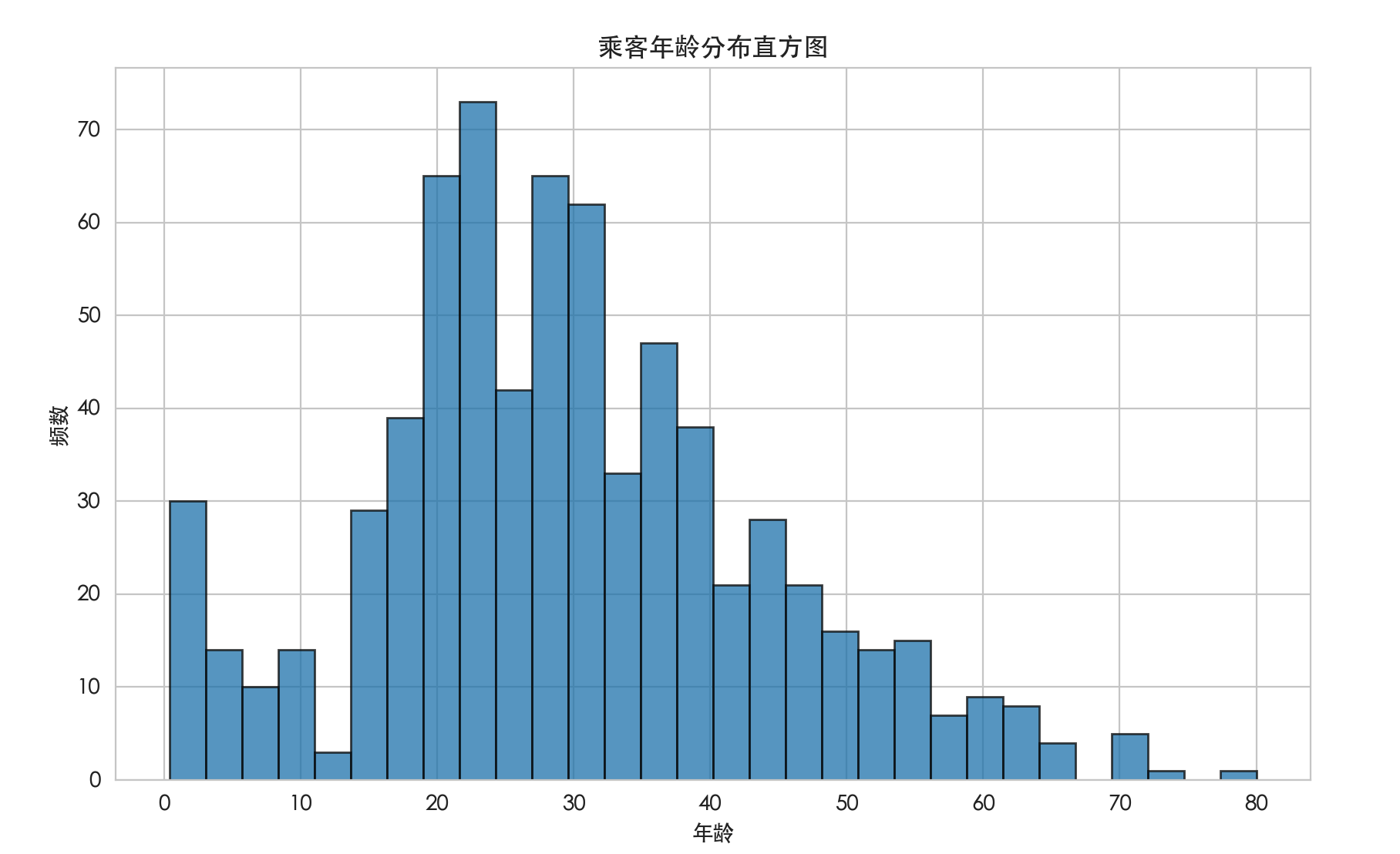
Interpretation: This chart can tell us in which interval the passengers' ages are mainly concentrated (e.g., 20-30 years), whether the distribution is symmetric, whether there are outliers, etc.
Box plotcan clearly show the data'smedian, quartiles, and outliers.。
Example
plt.figure(figsize=(8, 5))
plt.boxplot(df['fare'].dropna())
plt.title('Fare box plot')
plt.ylabel('Fare')
plt.show()
Interpretation: The line in the middle of the box is the median. The upper and lower edges of the box are the upper quartile (Q3) and lower quartile (Q1). The upper and lower "whiskers" usually extend to the furthest data points within 1.5 times the interquartile range; points beyond that are consideredoutliers(the circles above in the figure). This chart immediately tells us that there are many extremely high outliers in fare.
2. Categorical Features: Bar Charts
For features such assex(gender),embarked(port of embarkation),survived(survived or not) and other categorical features, we usebar chartsto count the number of each category.
Example
survival_counts = df['sex'].value_counts()
plt.figure(figsize=(8, 5))
plt.bar(survival_counts.index, survival_counts.values, color=['lightblue', 'lightcoral'])
plt.title('Passenger gender distribution')
plt.xlabel('Gender')
plt.ylabel('Count')
plt.show()
Bivariate Analysis: Exploring Relationships Between Features
Bivariate analysis exploresthe relationship between twofeatures.
1. Numerical vs Numerical: Scatter Plots
A scatter plot is a powerful tool for studying the correlation between two continuous variables.
Example
plt.figure(figsize=(10, 6))
plt.scatter(df['age'], df['fare'], alpha=0.5) # alpha sets the transparency to better observe point density
plt.title('Age vs Fare Scatter Plot')
plt.xlabel('Age')
plt.ylabel('Fare')
plt.show()
- Interpretation: The distribution pattern of the points can suggest correlation. For example, if the points roughly lie along a diagonal line, it indicates that the two variables are correlated. From this chart, age and fare do not show an obvious linear relationship, but it confirms again the existence of high fares (outliers).
2. Categorical vs Numerical: Grouped Box Plots or Violin Plots
We often want to know how the distribution of a numerical feature differs across categories. For example: "How does the fare distribution differ among passengers in different classes?"
Example
plt.figure(figsize=(10, 6))
sns.boxplot(x='pclass', y='fare', data=df)
plt.title('Fare distribution by passenger class')
plt.show()
- Interpretation: Very clear! Higher cabin class (First Class) has significantly higher median and overall range of ticket prices. This completely matches our common sense.
Violin plotis an advanced version of the box plot. It not only displays statistics but also shows the actual distribution shape of the data through kernel density estimation.
Example
plt.figure(figsize=(10, 6))
sns.violinplot(x='sex', y='age', data=df, inner='quartile') # The inner parameter displays quartile lines
plt.title('Age distribution by gender (violin plot)')
plt.show()
3. Categorical vs Categorical: Stacked Bar Charts or Heatmaps
For two categorical variables, we can usestacked bar chartsto observe the combination. For example: "What is the survival ratio by gender?"
Example
cross_tab = pd.crosstab(df['sex'], df['survived'], normalize='index') # normalize='index' calculates proportions by row
print(cross_tab)
# Draw a stacked bar chart
cross_tab.plot(kind='bar', stacked=True, figsize=(10, 6), color=['tomato', 'lightgreen'])
plt.title('Survival ratio by gender')
plt.xlabel('Gender')
plt.ylabel('Proportion')
plt.legend(['Not Survived', 'Survived'])
plt.show()
Interpretation: From the chart and crosstab, it is obvious that the survival ratio of women is much higher than that of men. This is a very strong signal indicating thatsexthe feature is crucial for predicting survival.
Multivariate Analysis and Advanced Visualization
Sometimes we need to consider three or even more variables at the same time.seabornThe library makes this easy.
1. Scatter Plot with Grouping
Based on a scatter plot, we can use color or shape to distinguish a third (categorical) variable.
Example
plt.figure(figsize=(12, 8))
sns.scatterplot(x='age', y='fare', hue='survived', style='survived', data=df, alpha=0.7)
plt.title('Age vs. Fare (colored by survival)')
plt.show()
- Interpretation: This chart lets us intuitively see whether the distributions of survivors (orange) and non-survivors (blue) differ in the two-dimensional space of "age-fare".
2. Correlation Matrix Heatmap
When we have multiple numeric features, we can compute the pairwise correlation coefficients at once and display them with a heatmap.
Example
numeric_df = df.select_dtypes(include=['float64', 'int64'])
# Compute the correlation coefficient matrix
corr_matrix = numeric_df.corr()
# Draw the heatmap
plt.figure(figsize=(12, 8))
sns.heatmap(corr_matrix, annot=True, cmap='coolwarm', center=0, square=True)
plt.title('Correlation matrix heatmap of numeric features')
plt.show()
Interpretation: Warmer colors (red) indicate stronger positive correlation; cooler colors (blue) indicate stronger negative correlation.annot=TrueDisplay the specific values inside the cells. For example,pclass(cabin class) andfare(fare) have a strong negative correlation (-0.55), meaning the smaller the class number (higher class), the higher the fare, which is consistent with our previous analysis.
Practical Exercise: Hands-On Exploration
Now, please try to complete the following exercises to consolidate what you have learned:
- Data inspection: Use
df.isnull().sum()to check which columns in the dataset have missing values and how many are missing. - Plot distribution: For the
agecolumn, draw aviolin plot, and group bysurvived(survival status) usingsns.violinplot(x='survived', y='age', data=df)). Observe how the age distributions of survivors and non-survivors differ. - Explore relationships: Use
sns.countplot(x='pclass', hue='survived', data=df)to draw a count bar chart and compare the number of survivors across different cabin classes. What conclusion can you draw? - (Challenge) Multivariate plot: Try to draw ascatter plot matrix, to view at once
age、fare、parch(parent/child count) and the pairwise relationships among these numeric variables. Hint: you can usesns.pairplot(df[['age', 'fare', 'parch', 'survived']], hue='survived')。
Summary
Data visualization is anindispensable exploratory stepin the machine learning workflow. Through this article, you have learned:
Core tools: Usematplotlibfor basic plotting, and useseabornto draw more beautiful and informative statistical graphics.
Analysis approach:
- Univariate analysis: Use histograms/box plots to see distributions, and bar charts to count frequencies.
- Bivariate analysis: Use scatter plots for numeric relationships, grouped box plots for the effect of categories on numeric values, and stacked bar charts for category combinations.
- Multivariate analysis: Use colored scatter plots and correlation heatmaps to reveal more complex patterns.
Core goal: All charts are intended topropose hypothesesandand discover insights, for example, gender may be an important predictive feature, and there are many outliers in the fare data that need to be handled.
Remember, before feeding data to a model, be sure to take time to look at it carefully. A clear insight from visualization can often guide you in the right direction earlier than complex algorithms.
Other Extensions Linux Command Reference