Loss Functions and Gradients
In this chapter, we will explore two crucial core concepts:Loss FunctionandGradient, which are the cornerstone that enables machine learning algorithms tolearnandimprove.
Imagine you are learning to shoot a basketball. After every shot, you observe whether the ball went in, veered left, or veered right. The gap between this observed result and a perfect shot is yourloss. To shoot more accurately next time, you adjust your posture and strength according to the direction and magnitude of this deviation. Thisdirection and magnitude of adjustmentis similar to thegradient。
In machine learning, the model is thelearner, the loss function measures itsdegree of error, and the gradient tells ithow to improve. Understanding these gives you the core logic of how machine learning works.
I. Loss Functions: The Model's Report Card
1.1 What is a loss function?
A loss function, sometimes calledcost functionorobjective function, is a function used toquantify the difference between model predictions and true values.
- Core role: It gives a concrete "score" to the model's prediction performance. The lower this score, the more accurate the model's predictions; the higher the score, the greater the prediction error.
- Analogy: Just like an exam, the "score" of the loss function is the model's exam grade. Our ultimate goal is to make this score (loss) lower and lower through "learning" (adjusting model parameters).
1.2 Examples of Common Loss Functions
Different tasks require differentscoring standards. Here are two of the most basic loss functions:
Mean Squared Error- Suitable for regression problems (predicting continuous values, such as house prices, temperature)
Mean squared error calculates theaverage of the squared differences between predicted values and true values across all samples。
Formula: MSE = (1/n) * Σ(真实值ᵢ - 预测值ᵢ)²
n: number of samplesΣ: summation symbolTrue valueᵢ: true value of the i-th samplePredicted valueᵢ: model's predicted value for the i-th sample
Characteristics: Because it uses squaring, it penalizes larger errors more heavily (when error is 2, the squared contribution is 4; when error is 10, the squared contribution is as high as 100).
Code Example:
Example
# Assume we have true and predicted values for 5 samples
y_true = np.array([3, -0.5, 2, 7, 4]) # True values
y_pred = np.array([2.5, 0.0, 2, 8, 5]) # Predicted values
# Manually compute MSE
n = len(y_true)
squared_errors = (y_true - y_pred) ** 2 # Calculate the squared error for each sample
mse_manual = np.sum(squared_errors) / n # Sum and take the average
print(f"MSE calculated manually: {mse_manual}")
# Verify using the sklearn library function
from sklearn.metrics import mean_squared_error
mse_sklearn = mean_squared_error(y_true, y_pred)
print(f"MSE calculated by Sklearn: {mse_sklearn}")
Cross-Entropy Loss- Suitable for classification problems (predicting categories, such as whether an image is a cat or a dog)
Cross-entropy measures the difference between theprobability distribution predicted by the modelandand the true probability distribution. In binary classification, the true distribution is usually[1, 0](is category A) or[0, 1](is category B).
Binary Classification Formula (Log Loss):
Log Loss = - (1/n) * Σ [真实值ᵢ * log(预测概率ᵢ) + (1 - 真实值ᵢ) * log(1 - 预测概率ᵢ)]
Intuitive understanding: When the true label is 1, we hope the probability predicted by the model is also close to 1. If the model predicts a very low probability (e.g., 0.1) at this point, thenlog(0.1)it will be a very large negative number; multiplying by the preceding negative sign causes the loss value to become very large, indicating a heavy penalty.
Code Example:
Example
from sklearn.metrics import log_loss
# Binary classification example: true labels (1 represents "yes", 0 represents "no")
y_true_binary = np.array([1, 0, 0, 1]) # True classes: yes, no, no, yes
# Probability predicted by the model for the "yes" class
y_pred_prob = np.array([0.9, 0.1, 0.2, 0.8]) # Predicted probabilities: 0.9, 0.1, 0.2, 0.8
# Use sklearn to compute cross-entropy loss (log loss)
ce_loss = log_loss(y_true_binary, y_pred_prob)
print(f"Cross-entropy loss (Log Loss): {ce_loss}")
II. Gradient: The "Compass" Guiding Optimization Direction
Now we know how to score the model (loss function). The next most critical question is:How does the model improve itself based on this score?The answer is through thegradient。
2.1 What is a gradient?
In machine learning, a model is usually composed of manyparameters(orweights). We can regard theloss function Las a function of all these parameters:L(w1, w2, ..., wn)。
- The gradientis the vector formed by thepartial derivativesofof the loss function with respect to each parameter.
- Mathematical Representation:
∇L = [∂L/∂w1, ∂L/∂w2, ..., ∂L/∂wn] - Core Meaning:
- Direction: The direction pointed by the gradient vector is the direction in which the loss functionincreases fastestat that point.
- Magnitude: The absolute value of each partial derivative represents thesensitivity。
2.2 Why can gradients guide optimization?
Our goal is tominimize the loss function. Since the gradient points in the direction where the loss increases fastest, its opposite direction-∇Lis naturally where the lossdecreases fastest.
The optimization process (gradient descent) can be vividly understood as:
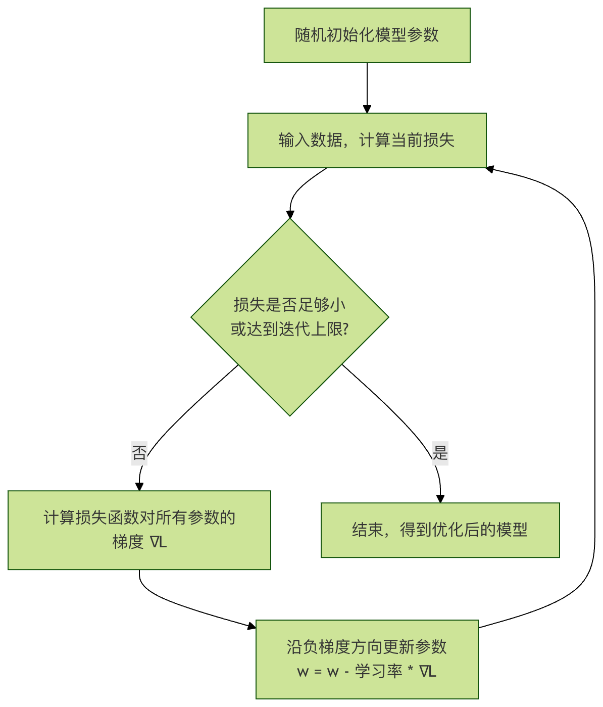
standing on a hillside of a valley (loss surface), blindfolded, wanting to reach the bottom of the valley (the point of minimum loss). Before each step, you use your feet to feel which direction around you is the steepest (compute the gradient), and then head toward the steepestdownhill direction(negative gradient direction) to take a step (update parameters). Repeating this process, you will eventually reach the bottom of the valley.
This process can be summarized by the following flowchart:
2.3 A Simple Example of Gradient Descent
Let's use a very simple example — a linear model with only one parameterwto demonstrate gradient descent.
Suppose our loss function isL(w) = w². Obviously, whenw = 0, the loss is minimized.
- Gradient Calculation:
∇L = dL/dw = 2w - Parameter Update Formula:
w_new = w_old - η * (2 * w_old)ηYesLearning rate, controls how large each step is.
Example
import matplotlib.pyplot as plt
# Define the loss function L(w) = w^2
def loss(w):
return w ** 2
# Define the gradient dL/dw = 2*w
def gradient(w):
return 2 * w
# Gradient descent algorithm
def gradient_descent(start_w, learning_rate, iterations):
w = start_w
w_history = [w] # Record the history of w changes
loss_history = [loss(w)] # Record the history of loss changes
for i in range(iterations):
grad = gradient(w) # Compute the gradient at the current point
w = w - learning_rate * grad # Update parameters along the negative gradient direction
w_history.append(w)
loss_history.append(loss(w))
return w_history, loss_history
# Run gradient descent: start from w=5, learning rate 0.1, iterate 20 times
w_start = 5.0
lr = 0.1
iters = 20
w_hist, loss_hist = gradient_descent(w_start, lr, iters)
print(f"Initial w: {w_hist)
print(f"Final w: {w_hist[-1]:.4f}, Final loss: {loss_hist[-1]:.4f}")
# Visualize the optimization process
plt.figure(figsize=(12, 4))
# Figure 1: Loss function curve and optimization path
plt.subplot(1, 2, 1)
w_vals = np.linspace(-6, 6, 100)
plt.plot(w_vals, loss(w_vals), label='L(w) = w²')
plt.scatter(w_hist, loss_hist, c='red', s=20, label='Gradient Descent Steps')
plt.plot(w_hist, loss_hist, 'r--', alpha=0.5)
plt.xlabel('Parameter w')
plt.ylabel('Loss L(w)')
plt.title('Gradient Descent on L(w)=w²')
plt.legend()
plt.grid(True)
# Figure 2: Loss value decline curve over iterations
plt.subplot(1, 2, 2)
plt.plot(range(len(loss_hist)), loss_hist, 'b-o')
plt.xlabel('Iteration')
plt.ylabel('Loss')
plt.title('Loss Reduction Over Iterations')
plt.grid(True)
plt.tight_layout()
plt.show()
Run this code, and you will see:
- the left figure shows how the parameter
wstarts from 5.0 and, step by step, "rolls down" the parabola, finally approaching the minimum point 0. - The right figure shows how the loss value decreases rapidly as the number of iterations increases.
III. Key Points and Relationship Summary
| Concept | Metaphor | Core Role | Key points |
|---|---|---|---|
| Loss function | Report card / error measuring ruler | Quantitatively evaluate how good or bad the model's predictions are. | 1. Different types of tasks (regression, classification) use different loss functions. 2. The smaller the loss value, the better the model performance. |
| Gradient | Compass / steepest downhill direction | Indicates how each model parameter should be adjusted to reduce loss most quickly. | 1. It is the vector of partial derivatives of the loss function with respect to all parameters. 2. Negative gradient directionIs the direction in which loss decreases fastest. |
| Gradient descent | Blindfolded downhill descent method | Uses gradient information to iteratively update parameters to minimize the loss. | 1. Learning rateIs a key hyperparameter; too small makes learning slow, too large may fail to converge. 2. It is the underlying optimization algorithm for training most machine learning models. |
The relationship chain between them is: Model makes predictions → Loss function computes the error → Compute the gradient of the error with respect to each parameter → Update parameters along the negative gradient direction → Model improves → Repeat...
Other extensions