R - Linear Regression

R Language Examples

In statistics, linear regression is a regression analysis that uses the least squares function, called the linear regression equation, to model the relationship between one or more independent variables and a dependent variable.

Simply put, it is a statistical analysis method used to determine the quantitative relationship of interdependence between two or more variables.

In regression analysis, if there is only one independent variable and one dependent variable, and the relationship between the two can be approximated by a straight line, this regression analysis is called simple linear regression analysis. If the regression analysis includes two or more independent variables and the relationship between the dependent variable and the independent variables is linear, it is called multiple linear regression analysis.

The mathematical equation for simple linear regression analysis:

y = ax + b

• yis the value of the dependent variable.

• xis the value of the independent variable.

• aandbare the parameters of the simple linear regression equation.

Next, we can create a prediction model for human height and weight:

• 1. Collect sample data: height and weight.
• 2. Use the lm() function to create a relationship model.
• 3. Find the coefficients from the created model and create a mathematical equation.
• 4. Obtain the summary of the relationship model to understand the average error, i.e., the residual (the difference between the estimated value and the true value).
• 5. Use the predict() function to predict a person's weight.

Prepare the data

The following is the height and weight data of people:

# 身高，单位 cm
151, 174, 138, 186, 128, 136, 179, 163, 152, 131

# 体重，单位 kg
63, 81, 56, 91, 47, 57, 76, 72, 62, 48

lm() Function

In R, you can perform linear regression using the lm() function.

The lm() function is used to create a relationship model between the independent variable and the dependent variable.

The syntax format of the lm() function is as follows:

lm(formula,data)

Parameter description:

• formula - a symbolic formula representing the relationship between x and y.
• data - the data to be applied.

Create a relationship model and obtain the coefficients:

Executing the above code outputs the result:

Call:
lm(formula = y ~ x)

Coefficients:
(Intercept)            x  
    -38.4551       0.6746  

Usesummary()the function to get the summary of the relationship model:

Executing the above code outputs the result:

Call:
lm(formula = y ~ x)

Residuals:
    Min      1Q     Median      3Q     Max 
-6.3002    -1.6629  0.0412    1.8944  3.9775 

Coefficients:
             Estimate Std. Error t value Pr(>|t|)    
(Intercept) -38.45509    8.04901  -4.778  0.00139 ** 
x             0.67461    0.05191  12.997 1.16e-06 ***
---
Signif. codes:  0 ‘***’ 0.001 ‘**’ 0.01 ‘*’ 0.05 ‘.’ 0.1 ‘ ’ 1

Residual standard error: 3.253 on 8 degrees of freedom
Multiple R-squared:  0.9548,    Adjusted R-squared:  0.9491 
F-statistic: 168.9 on 1 and 8 DF,  p-value: 1.164e-06

predict() Function

The predict() function is used to predict values based on the model we have built.

The syntax format of the predict() function is as follows:

predict(object, newdata)

Parameter description:

• object - the formula created by the lm() function.
• newdata - the value to be predicted.

In the following example, we predict a new weight value:

Executing the above code outputs the result:

1 
76.22869 

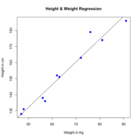
We can also generate a chart:

The chart is as follows:

R Language Examples