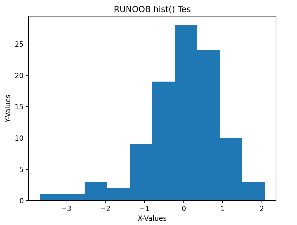
Matplotlib Histogram
We can use the `hist()` method in pyplot to draw histograms.
The `hist()` method is a function in the pyplot sub-library of the Matplotlib library used for drawing histograms.
The `hist()` method can be used to visualize the distribution of data, such as observing the central tendency, skewness, and outliers of the data.
The syntax of the `hist()` method is as follows:
matplotlib.pyplot.hist(x, bins=None, range=None, density=False, weights=None, cumulative=False, bottom=None, histtype='bar', align='mid', orientation='vertical', rwidth=None, log=False, color=None, label=None, stacked=False, **kwargs)
Parameter description:
x: Indicates the data used to draw the histogram, which can be a one-dimensional array or list.bins: Optional parameter, specifies the number of bins for the histogram. Default is 10.range: Optional parameter, specifies the value range of the histogram, which can be a tuple or list of two values. Default is None, meaning the minimum and maximum values in the data are used.density: Optional parameter, specifies whether to normalize the histogram. Default is False, meaning the height of the histogram is the number of samples in each bin, not the frequency or probability density.weights: Optional parameter, specifies the weight of each data point. Default is None.cumulative: Optional parameter, specifies whether to draw a cumulative distribution plot. Default is False.bottom: Optional parameter, specifies the bottom height of the histogram. Default is None.histtype: Optional parameter, specifies the type of histogram, which can be 'bar', 'barstacked', 'step', 'stepfilled', etc. Default is 'bar'.align: Optional parameter, specifies the alignment of histogram bins, which can be 'left', 'mid', or 'right'. Default is 'mid'.orientation: Optional parameter, specifies the orientation of the histogram, which can be 'vertical' or 'horizontal'. Default is 'vertical'.rwidth: Optional parameter, specifies the width of each bin. Default is None.log: Optional parameter, specifies whether to use a logarithmic scale on the y-axis. Default is False.color: Optional parameter, specifies the color of the histogram.label: Optional parameter, specifies the label of the histogram.stacked: Optional parameter, specifies whether to stack different histograms. Default is False.**kwargs: Optional parameter, other plotting parameters.
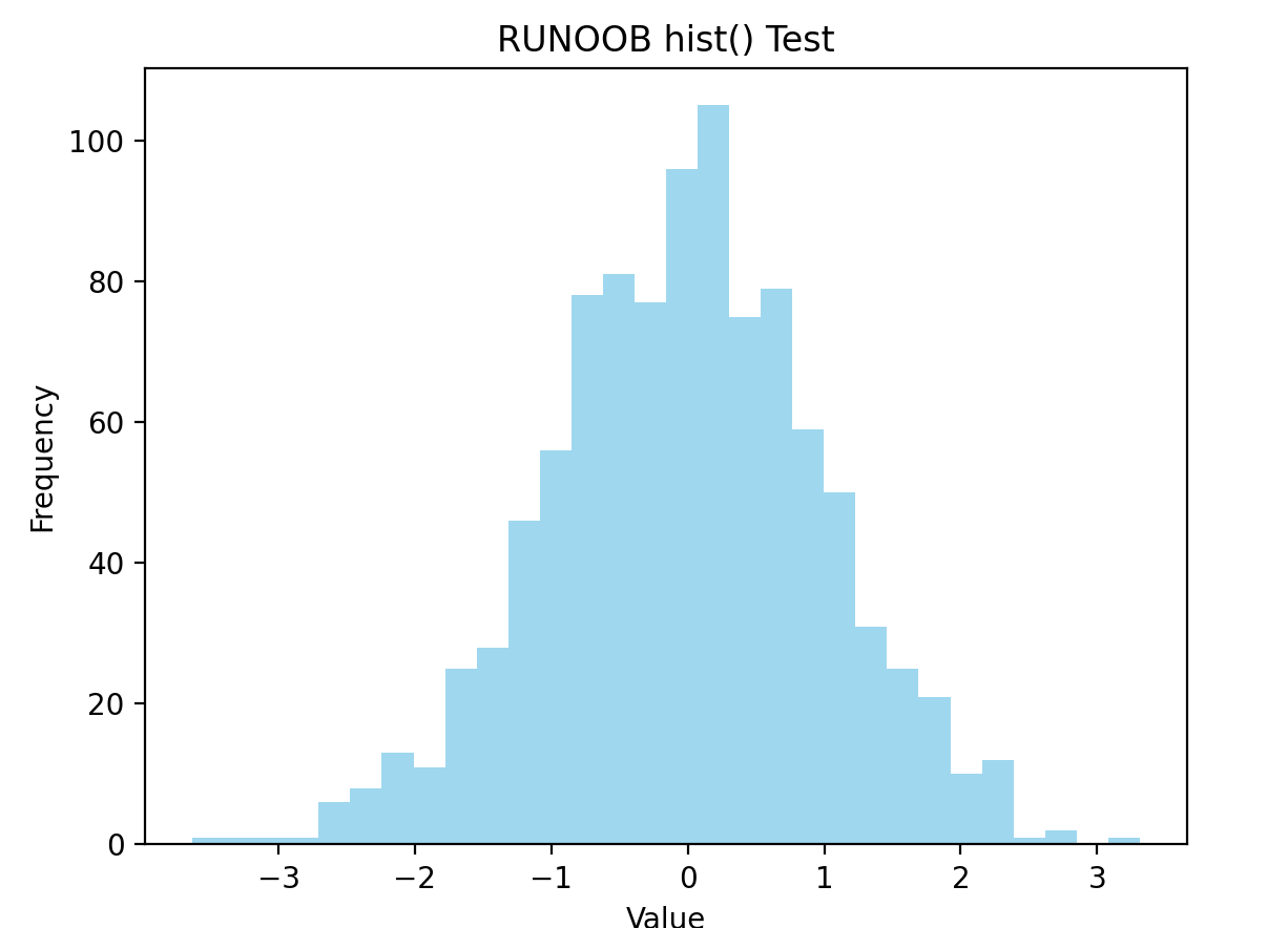
In the following example, we simply use `hist()` to create a histogram:
Example
import numpy as np
# Generate a set of random data
data = np.random.randn(1000)
# Draw the histogram
plt.hist(data, bins=30, color='skyblue', alpha=0.8)
# Set chart properties
plt.title('EXAMPLE hist() Test')
plt.xlabel('Value')
plt.ylabel('Frequency')
# Display the chart
plt.show()
The displayed result is as follows:
The following example demonstrates how to use the `hist()` function to draw histograms for multiple data groups and compare them:
Example
import numpy as np
# Generate three sets of random data
data1 = np.random.normal(0, 1, 1000)
data2 = np.random.normal(2, 1, 1000)
data3 = np.random.normal(-2, 1, 1000)
# Draw the histograms
plt.hist(data1, bins=30, alpha=0.5, label='Data 1')
plt.hist(data2, bins=30, alpha=0.5, label='Data 2')
plt.hist(data3, bins=30, alpha=0.5, label='Data 3')
# Set chart properties
plt.title('EXAMPLE hist() TEST')
plt.xlabel('Value')
plt.ylabel('Frequency')
plt.legend()
# Display the chart
plt.show()
In the above example, we generated three different sets of random data and used the `hist()` function to draw their histograms. By setting different means and standard deviations, we can generate random data with different distribution characteristics.
We set the `bins` parameter to 30, which means dividing the data range into 30 equal-width intervals, and then counting the frequency of data in each interval.
We set the `alpha` parameter to 0.5, which means the color transparency of each histogram is 50%.We used the `label` parameter to set the label of each histogram so that it can be displayed in the legend.
Then we use the `legend()` function to display the legend. Finally, we use the `title()`, `xlabel()`, and `ylabel()` functions to set the chart title and axis labels.
The displayed result is as follows:
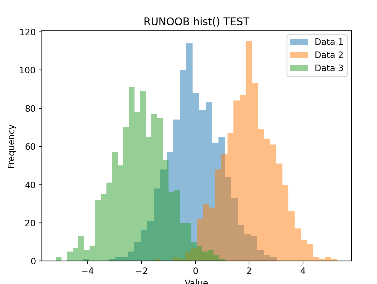
From the figure above, we can clearly see the distribution of these three data groups. Among them, `data1` and `data2` are close to a normal distribution, while `data3` is skewed.
This way of comparing histograms can help us analyze and compare the distribution of different data groups.
Combining with Pandas
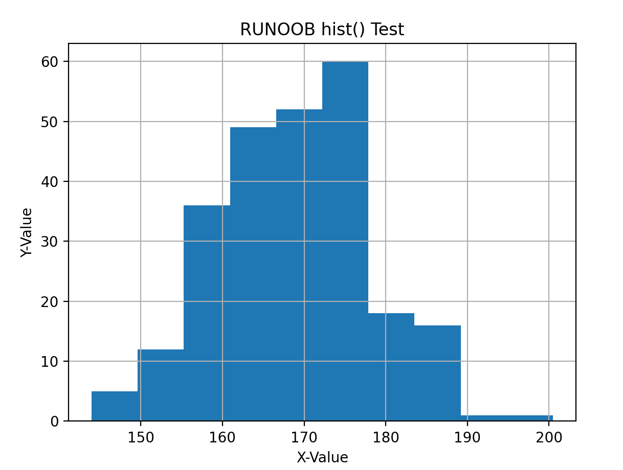
In the following example, we combine Pandas to draw a histogram:
Example
import pandas as pd
import matplotlib.pyplot as plt
# Use NumPy to generate random numbers
random_data = np.random.normal(170, 10, 250)
# Convert the data to a Pandas DataFrame
dataframe = pd.DataFrame(random_data)
# Use the Pandas hist() method to draw a histogram
dataframe.hist()
# Set chart properties
plt.title('EXAMPLE hist() Test')
plt.xlabel('X-Value')
plt.ylabel('Y-Value')
# Display the chart
plt.show()
The displayed result is as follows:
In addition to DataFrames, you can also use Series objects in Pandas to draw histograms. Simply replace the columns in the DataFrame with Series objects.
Example
import pandas as pd
import matplotlib.pyplot as plt
# Generate random data
data = pd.Series(np.random.normal(size=100))
# Draw the histogram
# The bins parameter specifies the number of bars in the histogram
plt.hist(data, bins=10)
# Set the chart title and axis labels
plt.title('EXAMPLE hist() Tes')
plt.xlabel('X-Values')
plt.ylabel('Y-Values')
# Display the chart
plt.show()