TensorFlow Model Tuning Tips
Model tuning is a crucial part of the machine learning workflow; it directly affects the final performance of the model. In TensorFlow, we can use a variety of technical methods to improve the model's accuracy and generalization ability.
Why Model Tuning is Needed
- Initial models are often not ideal: The first trained model often suffers from underfitting or overfitting
- Resource Utilization Optimization: Through tuning, better performance can be achieved with the same computing resources
- Business Requirements Matching: Different application scenarios have different requirements for models (e.g., accuracy vs. speed)
1.2 Main Tuning Directions
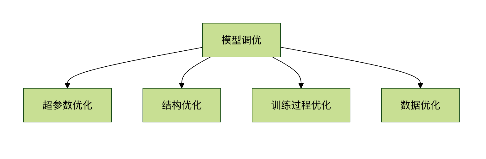
Hyperparameter Tuning Techniques
Learning Rate Adjustment
The learning rate is one of the most critical hyperparameters, directly affecting the model's convergence speed and final performance.
Static Learning Rate Setting
Example
optimizer = tf.keras.optimizers.Adam(learning_rate=0.001)
Dynamic Learning Rate Strategy
Example
initial_learning_rate = 0.1
lr_schedule = tf.keras.optimizers.schedules.ExponentialDecay(
initial_learning_rate,
decay_steps=10000,
decay_rate=0.96,
staircase=True)
optimizer = tf.keras.optimizers.SGD(learning_rate=lr_schedule)
Learning Rate Finder
Example
import keras_tuner as kt
def build_model(hp):
model = tf.keras.Sequential()
model.add(tf.keras.layers.Dense(10))
# Set learning rate search range
hp_learning_rate = hp.Choice('learning_rate', values=[1e-2, 1e-3, 1e-4])
model.compile(optimizer=tf.keras.optimizers.Adam(learning_rate=hp_learning_rate),
loss='mse')
return model
tuner = kt.RandomSearch(build_model, objective='val_loss', max_trials=5)
Batch Size Selection
Batch size affects training stability and memory usage:
| Batch Size | Advantages | Disadvantages |
|---|---|---|
| Small batch (16-64) | Fast convergence, good generalization | Unstable training |
| Medium batch (64-256) | Balanced choice | Requires more memory |
| Large batch (256+) | Stable training | May get stuck in local optima |
Model Structure Optimization
Layer Size and Depth Adjustment
Width Adjustment Techniques
Example
def build_model(hp):
model = tf.keras.Sequential()
# Search for the optimal number of neurons
hp_units = hp.Int('units', min_value=32, max_value=512, step=32)
model.add(tf.keras.layers.Dense(units=hp_units, activation='relu'))
model.add(tf.keras.layers.Dense(10))
model.compile(optimizer='adam', loss='mse')
return model
Depth Adjustment Strategies
1. Start with a shallow network and gradually increase depth.
2. Use residual connections (ResNet) to solve the vanishing gradient problem in deep networks.
Example
def residual_block(x, filters):
shortcut = x
x = tf.keras.layers.Conv2D(filters, (3,3), padding='same')(x)
x = tf.keras.layers.BatchNormalization()(x)
x = tf.keras.layers.Activation('relu')(x)
x = tf.keras.layers.Conv2D(filters, (3,3), padding='same')(x)
x = tf.keras.layers.BatchNormalization()(x)
x = tf.keras.layers.Add()([shortcut, x])
return tf.keras.layers.Activation('relu')(x)
Regularization Techniques
Dropout
Example
tf.keras.layers.Dense(128, activation='relu'),
tf.keras.layers.Dropout(0.5), # 50% of the neurons will be randomly dropped out
tf.keras.layers.Dense(10)
])
L1/L2 Regularization
Example
tf.keras.layers.Dense(64,
activation='relu',
kernel_regularizer=tf.keras.regularizers.l2(0.01))
Early Stopping
Example
monitor='val_loss',
patience=5, # Stop if validation loss does not improve for 5 consecutive epochs
restore_best_weights=True) # Restore the best weights
model.fit(x_train, y_train,
validation_data=(x_val, y_val),
epochs=100,
callbacks=[early_stopping])
Training Process Optimization
Data Augmentation
Example
data_augmentation = tf.keras.Sequential([
tf.keras.layers.RandomFlip("horizontal"),
tf.keras.layers.RandomRotation(0.1),
tf.keras.layers.RandomZoom(0.1),
])
# Train with augmented data
model.fit(data_augmentation(x_train), y_train, epochs=10)
Batch Normalization
Example
tf.keras.layers.Dense(64),
tf.keras.layers.BatchNormalization(),
tf.keras.layers.Activation('relu'),
tf.keras.layers.Dense(10)
])
Gradient Clipping
Example
optimizer = tf.keras.optimizers.Adam(clipvalue=1.0)
Advanced Tuning Techniques
Automated Hyperparameter Tuning
Example
tuner = kt.Hyperband(
build_model,
objective='val_accuracy',
max_epochs=10,
factor=3,
directory='my_dir',
project_name='intro_to_kt')
tuner.search(x_train, y_train, epochs=10, validation_data=(x_val, y_val))
best_model = tuner.get_best_models(num_models=1)[0]
Model Distillation
Example
teacher = tf.keras.models.load_model('teacher_model.h5')
# Student model definition
student = tf.keras.Sequential([...])
# Distillation loss
def distillation_loss(y_true, y_pred, teacher_pred, temp=5.0):
return tf.keras.losses.kl_divergence(
tf.nn.softmax(teacher_pred/temp),
tf.nn.softmax(y_pred/temp))
Practical Tuning Suggestions
- Establish a baseline: First train a simple model as a baseline.
- Adjust one parameter at a time: Avoid changing multiple parameters at the same time.
- Record experiments: Use TensorBoard or MLflow to track experiments.
- Validation set usage: Ensure the validation set represents the real data distribution.
- Consider computational cost: Balance tuning effectiveness with resource consumption.
Example
tensorboard_callback = tf.keras.callbacks.TensorBoard(log_dir="./logs")
model.fit(x_train, y_train, epochs=10, callbacks=[tensorboard_callback])
By systematically applying these tuning techniques, you can significantly improve the performance of TensorFlow models. Remember, model tuning is an iterative process that requires patience and careful experimental design.
Other Extensions