FFT (Fast Fourier Transform), also known as fast Fourier transform, is an efficient algorithm for DFT (Discrete Fourier Transform). It plays an irreplaceable role in digital processing methods based on time-frequency transform analysis.
FFT Principle
Formula Derivation
The DFT computation formula is:
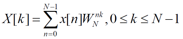
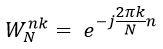
where,
By splitting the discrete Fourier transform formula into odd and even terms, the first N/2 points can be expressed as:
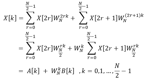
Similarly, the last N/2 points can be expressed as:

It can be seen that the values of the last N/2 points can be completely determined by the intermediate values obtained when calculating the first N/2 points. Continue to perform odd-even decomposition on A[k] and B[k] until it becomes a 2-point DFT, which avoids a lot of repeated calculations and realizes the fast discrete Fourier transform (FFT) process.
Algorithm Structure
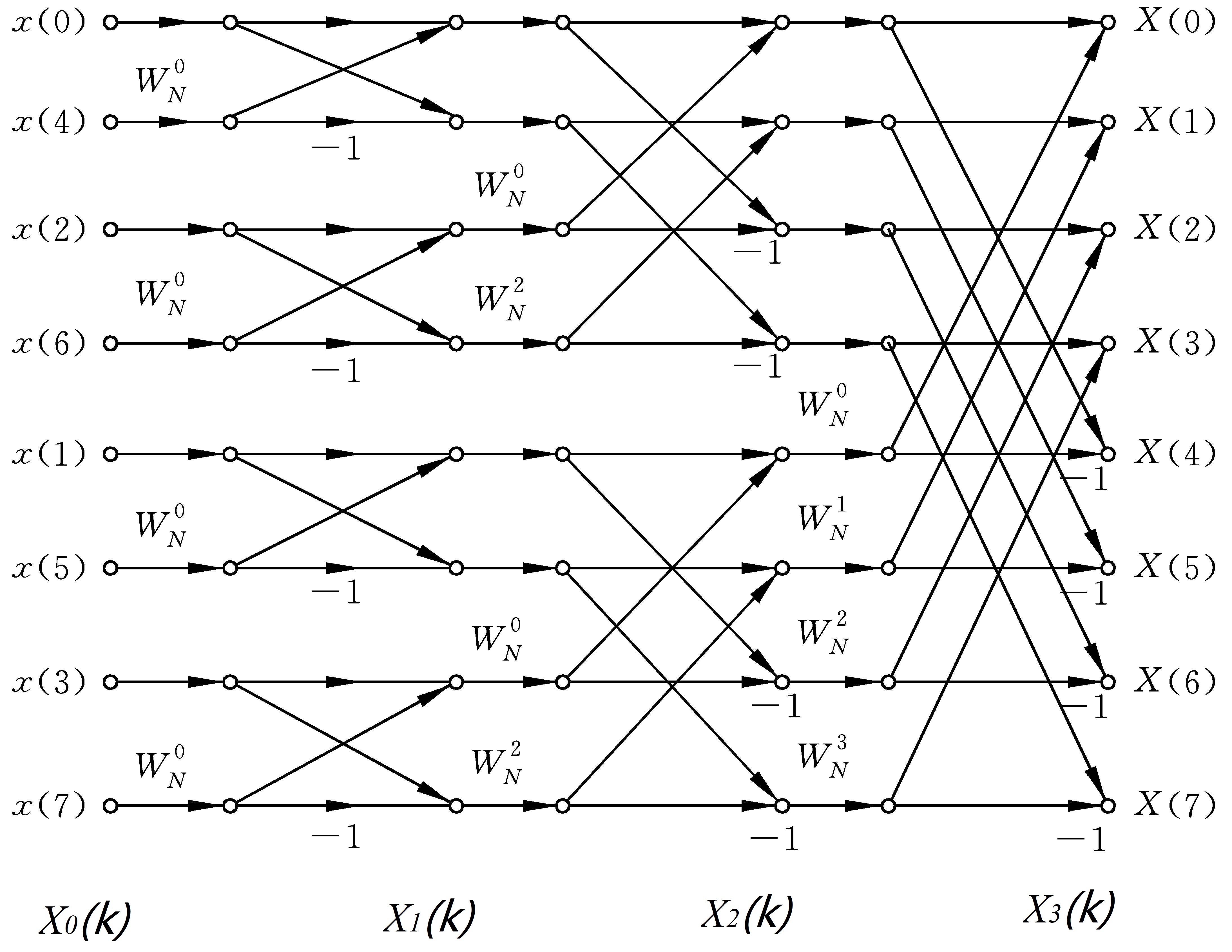
The structural diagram of the 8-point FFT computation is as follows.
It can be seen from the figure that the DFT process can be completed with only a few simple multiplications and additions, rather than tedious multiplication and accumulation for each data item.
Important Characteristics
(1) Concept of Stage
Each split is called one stage of operation.
Let the number of FFT operation points be N and the total number of stages be M; they satisfy:
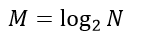
Each stage is identified by m = 0, 1, 2, ..., M-1.
To facilitate split computation, the number of FFT points N is often an integer power of 2.
(2) Butterfly Unit
The FFT computation structure consists of several butterfly operation units. The schematic diagram of each operation unit is as follows:
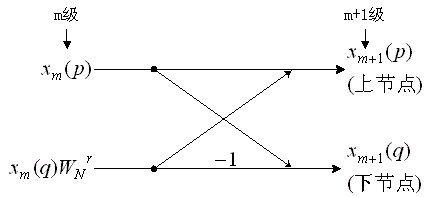
The input and output of the butterfly unit satisfy:
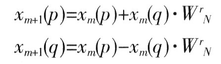
where,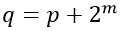
Each butterfly unit performs one multiplication and two additions during its operation.
Each stage has N/2 butterfly units.
Therefore, the number of multiplications and additions required to complete one FFT are respectively:

(3) Concept of Group
The N/2 butterfly units in each stage can be divided into several groups, and each group has the same structure and twiddle factor distribution.
For example, when m=0, it can be divided into N/2=4 groups.
When m=1, it can be divided into N/4=2 groups.
When m=M-1, it can only be divided into 1 group.
(4) Twiddle Factor Distribution The twiddle factor exists in stage m, where
 。
。
In the second stage of the 8-point FFT, i.e., m=1, the butterfly operation twiddle factor can be simplified to:

(5) Bit Reversal
For an N=8-point FFT computation, the binary codes corresponding to positions X(0) ~ X(7) are:
X(000), X(001), X(010), X(011), X(100), X(101), X(110), X(111)
Reverse the binary codes of their positions:
X(000), X(100), X(010), X(110), X(001), X(101), X(011), X(111)
The decimal values corresponding to the positions at this time are:
X(0), X(4), X(2), X(6), X(1), X(5), X(3), X(7)
This exactly corresponds to the order of the input data for the first stage of the FFT.
This characteristic is beneficial for the programming implementation of the FFT.
FFT Design
Design Description
In order to simply illustrate the FFT transformation process through simulation, the number of data points is set to a small value of 8.
If the data is input serially, it needs to be buffered first, so the data input method in this design is parallel.
The data input is divided into two parts: real part and imaginary part, so the calculation results are also divided into real part and imaginary part.
The design adopts a pipeline structure and does not consider resource consumption for now.
To make the design structure simpler, a compromise is made here: the multiplication calculation directly uses the multiplication operator. If the FFT design is applied in practice, the multiplication structure must be replaced with a pipelined multiplier, or use the official high-efficiency multiplier IP.
Butterfly Unit Design
The butterfly unit uses fixed-point operations, so the twiddle factor needs to be quantized to fixed-point.
Use MATLAB to multiply the twiddle factor by 8192 (left shift by 13 bits); see the appendix.
To prevent the multiplication and addition in butterfly operations from increasing the bit width stage by stage, after each stage of operation, the output data must be truncated to a fixed bit width. This also removes the effect of the twiddle factor scaling. The code is as follows:
Example
/**************** butter unit *************************
Xm(p) ------------------------> Xm+1(p)
- ->
- -
-
- -
- ->
Xm(q) ------------------------> Xm+1(q)
Wn -1
*//////////////////////////////////////////////////////
module butterfly
(
input clk,
input rstn,
input en,
input signed [23:0] xp_real, // Xm(p)
input signed [23:0] xp_imag,
input signed [23:0] xq_real, // Xm(q)
input signed [23:0] xq_imag,
input signed [15:0] factor_real, // Wnr
input signed [15:0] factor_imag,
output valid,
output signed [23:0] yp_real, //Xm+1(p)
output signed [23:0] yp_imag,
output signed [23:0] yq_real, //Xm+1(q)
output signed [23:0] yq_imag);
reg [4:0] en_r ;
always @(posedge clk or negedge rstn) begin
if (!rstn) begin
en_r <= 'b0 ;
end
else begin
en_r <= {en_r[3:0], en} ;
end
end
//=====================================================//
//(1.0) Xm(q) mutiply and Xm(p) delay
reg signed [39:0] xq_wnr_real0;
reg signed [39:0] xq_wnr_real1;
reg signed [39:0] xq_wnr_imag0;
reg signed [39:0] xq_wnr_imag1;
reg signed [39:0] xp_real_d;
reg signed [39:0] xp_imag_d;
always @(posedge clk or negedge rstn) begin
if (!rstn) begin
xp_real_d <= 'b0;
xp_imag_d <= 'b0;
xq_wnr_real0 <= 'b0;
xq_wnr_real1 <= 'b0;
xq_wnr_imag0 <= 'b0;
xq_wnr_imag1 <= 'b0;
end
else if (en) begin
xq_wnr_real0 <= xq_real * factor_real;
xq_wnr_real1 <= xq_imag * factor_imag;
xq_wnr_imag0 <= xq_real * factor_imag;
xq_wnr_imag1 <= xq_imag * factor_real;
//expanding 8192 times as Wnr
xp_real_d <= {{4{xp_real[23]}}, xp_real[22:0], 13'b0};
xp_imag_d <= {{4{xp_imag[23]}}, xp_imag[22:0], 13'b0};
end
end
//(1.1) get Xm(q) mutiplied-results and Xm(p) delay again
reg signed [39:0] xp_real_d1;
reg signed [39:0] xp_imag_d1;
reg signed [39:0] xq_wnr_real;
reg signed [39:0] xq_wnr_imag;
always @(posedge clk or negedge rstn) begin
if (!rstn) begin
xp_real_d1 <= 'b0;
xp_imag_d1 <= 'b0;
xq_wnr_real <= 'b0 ;
xq_wnr_imag <= 'b0 ;
end
else if (en_r[0]) begin
xp_real_d1 <= xp_real_d;
xp_imag_d1 <= xp_imag_d;
// Set bit width margin in advance to prevent data overflow
xq_wnr_real <= xq_wnr_real0 - xq_wnr_real1 ;
xq_wnr_imag <= xq_wnr_imag0 + xq_wnr_imag1 ;
end
end
//======================================================//
//(2.0) butter results
reg signed [39:0] yp_real_r;
reg signed [39:0] yp_imag_r;
reg signed [39:0] yq_real_r;
reg signed [39:0] yq_imag_r;
always @(posedge clk or negedge rstn) begin
if (!rstn) begin
yp_real_r <= 'b0;
yp_imag_r <= 'b0;
yq_real_r <= 'b0;
yq_imag_r <= 'b0;
end
else if (en_r[1]) begin
yp_real_r <= xp_real_d1 + xq_wnr_real;
yp_imag_r <= xp_imag_d1 + xq_wnr_imag;
yq_real_r <= xp_real_d1 - xq_wnr_real;
yq_imag_r <= xp_imag_d1 - xq_wnr_imag;
end
end
//(3) discard the low 13bits because of Wnr
assign yp_real = {yp_real_r[39], yp_real_r[13+23:13]};
assign yp_imag = {yp_imag_r[39], yp_imag_r[13+23:13]};
assign yq_real = {yq_real_r[39], yq_real_r[13+23:13]};
assign yq_imag = {yq_imag_r[39], yq_imag_r[13+23:13]};
assign valid = en_r[2];
endmodule
Top-Level Instantiation
According to the FFT algorithm structure diagram, instantiate the butterfly units to complete the final FFT function.
You can manually instantiate 12 times in sequence according to the input-output correspondence of the butterfly units in each stage, or use generate for instantiation. In that case, you need to be very familiar with the characteristics of "groups" and "stages" in the FFT:
-
(1) An 8-point FFT design requires 3 stages of operation. Each stage has 4 butterfly units, and the number of groups in each stage is 4, 2, 1 respectively.
-
(2) In each stage, the distance between the two input ports of a butterfly unit within a group is always
 (m is the stage index, corresponding to the left shift operation 1<<m); the distance between the first input ports of the two butterfly units in a group is 1.
 -
(3) The distance between the first input ports of the first butterfly units of adjacent groups in each stage is
 (corresponding to the left shift operation 2<<m).
The instantiation code is as follows.
Here, the one-dimensional and two-dimensional addresses of the matrix signals xm_real (xm_imag) are identifiers representing the stage and group.
When determining the connection relationships between signal ports, seemingly complex judgment logic is used, and it also contains multiplication operators. In fact, the final generated circuit is exactly the same as manually writing code to instantiate 12 butterfly units. This is because the variables in the generate block only assist in generating the actual circuit, and the calculation and judgment of related values are completed at compile time. These variables certainly do not generate actual circuits; they only provide a method for faster module instantiation.
Example
module fft8 (
input clk,
input rstn,
input en,
input signed [23:0] x0_real,
input signed [23:0] x0_imag,
input signed [23:0] x1_real,
input signed [23:0] x1_imag,
input signed [23:0] x2_real,
input signed [23:0] x2_imag,
input signed [23:0] x3_real,
input signed [23:0] x3_imag,
input signed [23:0] x4_real,
input signed [23:0] x4_imag,
input signed [23:0] x5_real,
input signed [23:0] x5_imag,
input signed [23:0] x6_real,
input signed [23:0] x6_imag,
input signed [23:0] x7_real,
input signed [23:0] x7_imag,
output valid,
output signed [23:0] y0_real,
output signed [23:0] y0_imag,
output signed [23:0] y1_real,
output signed [23:0] y1_imag,
output signed [23:0] y2_real,
output signed [23:0] y2_imag,
output signed [23:0] y3_real,
output signed [23:0] y3_imag,
output signed [23:0] y4_real,
output signed [23:0] y4_imag,
output signed [23:0] y5_real,
output signed [23:0] y5_imag,
output signed [23:0] y6_real,
output signed [23:0] y6_imag,
output signed [23:0] y7_real,
output signed [23:0] y7_imag
);
//operating data
wire signed [23:0] xm_real [3:0] [7:0];
wire signed [23:0] xm_imag [3:0] [7:0];
wire en_connect [15:0] ;
assign en_connect[0] = en;
assign en_connect[1] = en;
assign en_connect[2] = en;
assign en_connect[3] = en;
//factor, multiplied by 0x2000
wire signed [15:0] factor_real [3:0] ;
wire signed [15:0] factor_imag [3:0];
assign factor_real[0] = 16'h2000; //1
assign factor_imag[0] = 16'h0000; //0
assign factor_real[1] = 16'h16a0; //sqrt(2)/2
assign factor_imag[1] = 16'he95f; //-sqrt(2)/2
assign factor_real[2] = 16'h0000; //0
assign factor_imag[2] = 16'he000; //-1
assign factor_real[3] = 16'he95f; //-sqrt(2)/2
assign factor_imag[3] = 16'he95f; //-sqrt(2)/2
// Input initialization; related to bit reversal
assign xm_real[0][0] = x0_real;
assign xm_real[0][1] = x4_real;
assign xm_real[0][2] = x2_real;
assign xm_real[0][3] = x6_real;
assign xm_real[0][4] = x1_real;
assign xm_real[0][5] = x5_real;
assign xm_real[0][6] = x3_real;
assign xm_real[0][7] = x7_real;
assign xm_imag[0][0] = x0_imag;
assign xm_imag[0][1] = x4_imag;
assign xm_imag[0][2] = x2_imag;
assign xm_imag[0][3] = x6_imag;
assign xm_imag[0][4] = x1_imag;
assign xm_imag[0][5] = x5_imag;
assign xm_imag[0][6] = x3_imag;
assign xm_imag[0][7] = x7_imag;
//butter instantiaiton
//integer index[11:0] ;
genvar m, k;
generate
//3 stage
for(m=0; m<=2; m=m+1) begin: stage
for (k=0; k<=3; k=k+1) begin: unit
butterfly u_butter(
.clk (clk ) ,
.rstn (rstn ) ,
.en (en_connect[m*4 + k] ) ,
// Whether within the group? group index + intra-group index : next group index + new intra-group index
.xp_real (xm_real[ m ] [k[m:0] < (1<<m) ?
(k[3:m] << (m+1)) + k[m:0] :
(k[3:m] << (m+1)) + (k[m:0]-(1<<m))] ),
.xp_imag (xm_imag[ m ] [k[m:0] < (1<<m) ?
(k[3:m] << (m+1)) + k[m:0] :
(k[3:m] << (m+1)) + (k[m:0]-(1<<m))] ),
.xq_real (xm_real[ m ] [(k[m:0] < (1<<m) ?
(k[3:m] << (m+1)) + k[m:0] :
(k[3:m] << (m+1)) + (k[m:0]-(1<<m))) + (1<<m) ]), // Increase the distance between the two input ports of the butterfly unit
.xq_imag (xm_imag[ m ] [(k[m:0] < (1<<m) ?
(k[3:m] << (m+1)) + k[m:0] :
(k[3:m] << (m+1)) + (k[m:0]-(1<<m))) + (1<<m) ]),
.factor_real(factor_real[k[m:0]<(1<<m)?
k[m:0] : k[m:0]-(1<<m) ]),
.factor_imag(factor_imag[k[m:0]<(1<<m)?
k[m:0] : k[m:0]-(1<<m) ]),
//output data
.valid (en_connect[ (m+1)*4 + k ] ),
.yp_real (xm_real[ m+1 ][k[m:0] < (1<<m) ?
(k[3:m] << (m+1)) + k[m:0] :
(k[3:m] << (m+1)) + (k[m:0]-(1<<m))] ),
.yp_imag (xm_imag[ m+1 ][(k[m:0]) < (1<<m) ?
(k[3:m] << (m+1)) + k[m:0] :
(k[3:m] << (m+1)) + (k[m:0]-(1<<m))] ),
.yq_real (xm_real[ m+1 ][(k[m:0] < (1<<m) ?
(k[3:m] << (m+1)) + k[m:0] :
(k[3:m] << (m+1)) + (k[m:0]-(1<<m))) + (1<<m) ]),
.yq_imag (xm_imag[ m+1 ][((k[m:0]) < (1<<m) ?
(k[3:m] << (m+1)) + k[m:0] :
(k[3:m] << (m+1)) + (k[m:0]-(1<<m))) + (1<<m) ])
);
end
end
endgenerate
assign valid = en_connect[12];
assign y0_real = xm_real[3][0] ;
assign y0_imag = xm_imag[3][0] ;
assign y1_real = xm_real[3][1] ;
assign y1_imag = xm_imag[3][1] ;
assign y2_real = xm_real[3][2] ;
assign y2_imag = xm_imag[3][2] ;
assign y3_real = xm_real[3][3] ;
assign y3_imag = xm_imag[3][3] ;
assign y4_real = xm_real[3][4] ;
assign y4_imag = xm_imag[3][4] ;
assign y5_real = xm_real[3][5] ;
assign y5_imag = xm_imag[3][5] ;
assign y6_real = xm_real[3][6] ;
assign y6_imag = xm_imag[3][6] ;
assign y7_real = xm_real[3][7] ;
assign y7_imag = xm_imag[3][7] ;
endmodule
testbench
The testbench is written as follows, mainly for continuous input of 16 channels of real and complex data. Since each FFT has only 8 data points, the input data are arbitrary, not regular data such as sine waves.
Example
module test ;
reg clk;
reg rstn;
reg en ;
reg signed [23:0] x0_real;
reg signed [23:0] x0_imag;
reg signed [23:0] x1_real;
reg signed [23:0] x1_imag;
reg signed [23:0] x2_real;
reg signed [23:0] x2_imag;
reg signed [23:0] x3_real;
reg signed [23:0] x3_imag;
reg signed [23:0] x4_real;
reg signed [23:0] x4_imag;
reg signed [23:0] x5_real;
reg signed [23:0] x5_imag;
reg signed [23:0] x6_real;
reg signed [23:0] x6_imag;
reg signed [23:0] x7_real;
reg signed [23:0] x7_imag;
wire valid;
wire signed [23:0] y0_real;
wire signed [23:0] y0_imag;
wire signed [23:0] y1_real;
wire signed [23:0] y1_imag;
wire signed [23:0] y2_real;
wire signed [23:0] y2_imag;
wire signed [23:0] y3_real;
wire signed [23:0] y3_imag;
wire signed [23:0] y4_real;
wire signed [23:0] y4_imag;
wire signed [23:0] y5_real;
wire signed [23:0] y5_imag;
wire signed [23:0] y6_real;
wire signed [23:0] y6_imag;
wire signed [23:0] y7_real;
wire signed [23:0] y7_imag;
initial begin
clk = 0; //50MHz
rstn = 0 ;
#10 rstn = 1;
forever begin
#10 clk = ~clk; //50MHz
end
end
fft8 u_fft (
.clk (clk ),
.rstn (rstn ),
.en (en ),
.x0_real (x0_real),
.x0_imag (x0_imag),
.x1_real (x1_real),
.x1_imag (x1_imag),
.x2_real (x2_real),
.x2_imag (x2_imag),
.x3_real (x3_real),
.x3_imag (x3_imag),
.x4_real (x4_real),
.x4_imag (x4_imag),
.x5_real (x5_real),
.x5_imag (x5_imag),
.x6_real (x6_real),
.x6_imag (x6_imag),
.x7_real (x7_real),
.x7_imag (x7_imag),
.valid (valid),
.y0_real (y0_real),
.y0_imag (y0_imag),
.y1_real (y1_real),
.y1_imag (y1_imag),
.y2_real (y2_real),
.y2_imag (y2_imag),
.y3_real (y3_real),
.y3_imag (y3_imag),
.y4_real (y4_real),
.y4_imag (y4_imag),
.y5_real (y5_real),
.y5_imag (y5_imag),
.y6_real (y6_real),
.y6_imag (y6_imag),
.y7_real (y7_real),
.y7_imag (y7_imag));
//data input
initial begin
en = 0 ;
x0_real = 24'd10;
x1_real = 24'd20;
x2_real = 24'd30;
x3_real = 24'd40;
x4_real = 24'd10;
x5_real = 24'd20;
x6_real = 24'd30;
x7_real = 24'd40;
x0_imag = 24'd0;
x1_imag = 24'd0;
x2_imag = 24'd0;
x3_imag = 24'd0;
x4_imag = 24'd0;
x5_imag = 24'd0;
x6_imag = 24'd0;
x7_imag = 24'd0;
@(negedge clk) ;
en = 1 ;
forever begin
@(negedge clk) ;
x0_real = (x0_real > 22'h3F_ffff) ? 'b0 : x0_real + 1 ;
x1_real = (x1_real > 22'h3F_ffff) ? 'b0 : x1_real + 1 ;
x2_real = (x2_real > 22'h3F_ffff) ? 'b0 : x2_real + 31 ;
x3_real = (x3_real > 22'h3F_ffff) ? 'b0 : x3_real + 1 ;
x4_real = (x4_real > 22'h3F_ffff) ? 'b0 : x4_real + 23 ;
x5_real = (x5_real > 22'h3F_ffff) ? 'b0 : x5_real + 1 ;
x6_real = (x6_real > 22'h3F_ffff) ? 'b0 : x6_real + 6 ;
x7_real = (x7_real > 22'h3F_ffff) ? 'b0 : x7_real + 1 ;
x0_imag = (x0_imag > 22'h3F_ffff) ? 'b0 : x0_imag + 2 ;
x1_imag = (x1_imag > 22'h3F_ffff) ? 'b0 : x1_imag + 5 ;
x2_imag = (x2_imag > 22'h3F_ffff) ? 'b0 : x2_imag + 3 ;
x3_imag = (x3_imag > 22'h3F_ffff) ? 'b0 : x3_imag + 6 ;
x4_imag = (x4_imag > 22'h3F_ffff) ? 'b0 : x4_imag + 4 ;
x5_imag = (x5_imag > 22'h3F_ffff) ? 'b0 : x5_imag + 8 ;
x6_imag = (x6_imag > 22'h3F_ffff) ? 'b0 : x6_imag + 11 ;
x7_imag = (x7_imag > 22'h3F_ffff) ? 'b0 : x7_imag + 7 ;
end
end
//finish simulation
initial #1000 $finish ;
endmodule
Simulation Results
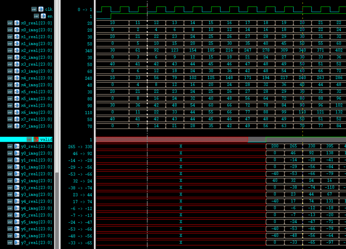
It can be roughly seen that the FFT results can be output in a pipeline manner.
Using MATLAB's built-in FFT function to operate on the same data, the FFT results of the first 2 groups of data are as follows.
It can be seen that when the first input data signal has only the real part valid, the FFT results are exactly the same.
However, when the second input data also has a signal in the imaginary part, the results between the two begin to have errors, and sometimes the errors are quite large.
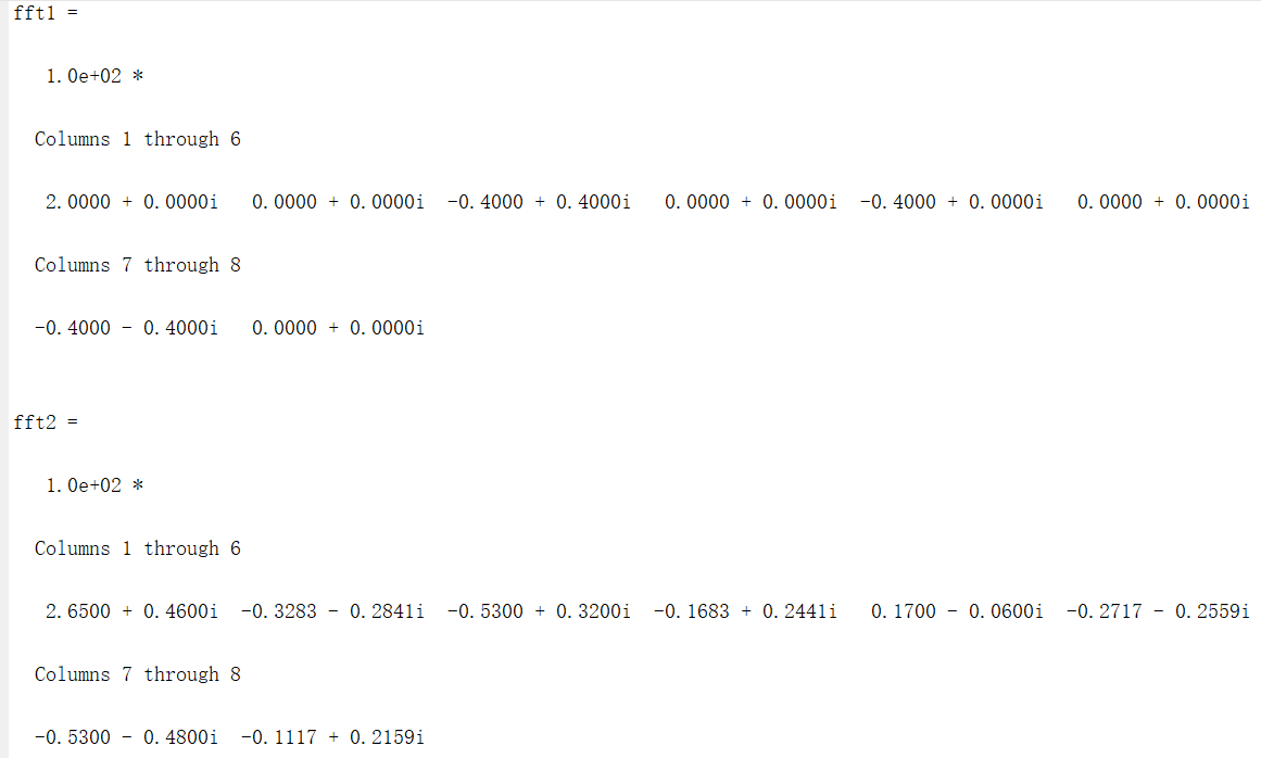
Using MATLAB to simulate the FFT process implemented in Verilog, it is found that the FFT results of this process are basically consistent with the FFT results implemented in Verilog.
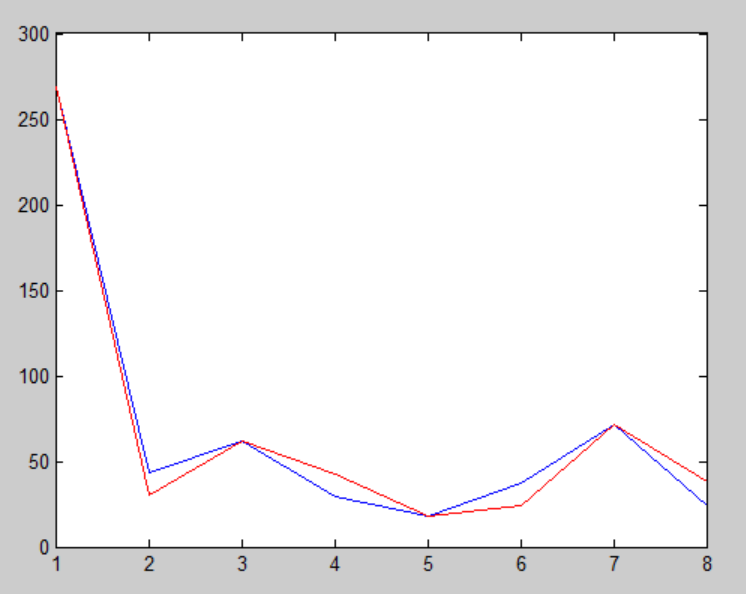
Take the absolute values of the two erroneous FFT results for comparison, as shown in the figure below.
It can be seen that the trends of the FFT results are roughly the same, but there are visible errors at individual points.
Design Summary:
As mentioned in the butterfly unit design, when quantizing the twiddle factor, the choice of bit width introduces errors.
Moreover, the operation result of each butterfly unit is truncated, which also introduces errors.
MATLAB does not need to consider precision issues when calculating FFT; it performs FFT calculations on the data with its highest precision.
All of the above will lead to differences between the results of the two FFT calculation methods.
Interested readers can further increase the bit widths of the twiddle factor and input data, and can also increase the number of FFT points, then perform simulation comparison; the relative error should decrease.
Appendix: MATLAB Usage
Generate Twiddle Factors
An 8-point FFT only needs 4 twiddle factors. The twiddle factors are scaled by 8192.
Example
%=======================================================
% Wnr calcuting
%=======================================================
for r = 0:3
Wnr_factor = cos(pi/4*r) - j*sin(pi/4*r) ;
Wnr_integer = floor(Wnr_factor * 2^13) ;
if (real(Wnr_integer)<0)
Wnr_real = real(Wnr_integer) + 2^16 ; %Two's Complement of Negative Numbers
else
Wnr_real = real(Wnr_integer) ;
end
if (imag(Wnr_integer)<0)
Wnr_imag = imag(Wnr_integer) + 2^16 ;
else
Wnr_imag = imag(Wnr_integer);
end
Wnr(2*r+1,:) = dec2hex(Wnr_real) %Real Part
Wnr(2*r+2,:) = dec2hex(Wnr_imag) %Imaginary Part
end
FFT Result Comparison
The MATLAB simulation of the FFT process implemented in Verilog is as follows, and it also includes a comparison of the two FFT results.
Example
%=======================================================
% 8dots fft
%=======================================================
for r=0:3
Wnr(r+1) = cos(pi/4*r) - j*sin(pi/4*r) ;
end
x = [10, 20, 30, 40, 10, 20 ,30 ,40];
step = [1+2j, 1+5j, 31+3j, 1+6j, 23+4j, 1+8j, 6+11j, 1+7j];
x2 = x + step;
xm0 = [x2(0+1), x2(4+1), x2(2+1), x2(6+1), x2(1+1), x2(5+1), x2(3+1), x2(7+1)] ;
%% stage1
xm1(1) = xm0(1) + xm0(2)*Wnr(1) ;
xm1(2) = xm0(1) - xm0(2)*Wnr(1) ;
xm1(3) = xm0(3) + xm0(4)*Wnr(1) ;
xm1(4) = xm0(3) - xm0(4)*Wnr(1) ;
xm1(5) = xm0(5) + xm0(6)*Wnr(1) ;
xm1(6) = xm0(5) - xm0(6)*Wnr(1) ;
xm1(7) = xm0(7) + xm0(8)*Wnr(1) ;
xm1(8) = xm0(7) - xm0(8)*Wnr(1) ;
floor(xm1(:))
%% stage2
xm2(1) = xm1(1) + xm1(3)*Wnr(1) ;
xm2(3) = xm1(1) - xm1(3)*Wnr(1) ;
xm2(2) = xm1(2) + xm1(4)*Wnr(2) ;
xm2(4) = xm1(2) - xm1(4)*Wnr(2) ;
xm2(5) = xm1(5) + xm1(7)*Wnr(1) ;
xm2(7) = xm1(5) - xm1(7)*Wnr(1) ;
xm2(6) = xm1(6) + xm1(8)*Wnr(2) ;
xm2(8) = xm1(6) - xm1(8)*Wnr(2) ;
floor(xm2(:))
%% stage3
xm3(1) = xm2(1) + xm2(5)*Wnr(1) ;
xm3(5) = xm2(1) - xm2(5)*Wnr(1) ;
xm3(2) = xm2(2) + xm2(6)*Wnr(2) ;
xm3(6) = xm2(2) - xm2(6)*Wnr(2) ;
xm3(3) = xm2(3) + xm2(7)*Wnr(3) ;
xm3(7) = xm2(3) - xm2(7)*Wnr(3) ;
xm3(4) = xm2(4) + xm2(8)*Wnr(4) ;
xm3(8) = xm2(4) - xm2(8)*Wnr(4) ;
floor(xm3(:))
%% fft
fft1 = fft(x)
fft2 = fft(x2)
plot(1:8, abs(fft2))
hold on
plot(1:8, abs(xm3), 'r')
Source Code Download
Download