Data Processing Tools
Natural Language Processing (NLP) is an important branch of artificial intelligence, and data processing is the key to the success of NLP projects.
This article will systematically introduce the essential toolset for the entire NLP data processing workflow, covering core stages such as data cleaning, numerical computation, feature engineering, machine learning, and visualization.
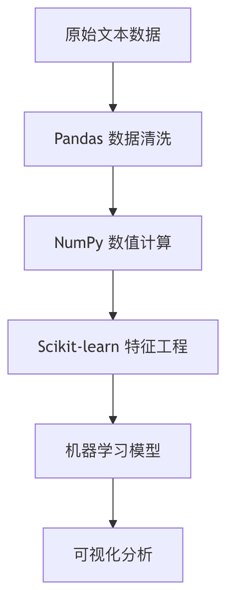
Pandas: Data Cleaning and Preprocessing
Pandas Core Data Structures
Pandas provides two main data structures, which are the cornerstone of NLP data processing:
| Data Structure | Features | NLP Application Scenarios |
|---|---|---|
| Series | One-dimensional labeled array | Store a single text feature column |
| DataFrame | Two-dimensional tabular structure | Store the entire text dataset |
Common Text Processing Operations
Example
# Create sample data
data = {'text': ['Hello World!', 'NLP is amazing', 'Python 3.8'],
'label': [1, 0, 1]}
df = pd.DataFrame(data)
# 1. Text cleaning
df['clean_text'] = df['text'].str.lower() # Convert to lowercase
df['clean_text'] = df['clean_text'].str.replace('[^\w\s]', '') # Remove punctuation
# 2. Tokenization
df['tokens'] = df['clean_text'].str.split() # Tokenize by spaces
# 3. Word frequency counting
word_counts = df['tokens'].explode().value_counts()
print(word_counts)
Advanced Text Processing Techniques
- Regular expression filtering:
df['text'].str.contains(r'\bNLP\b') - Stop word removal: using NLTK or spaCy libraries
- Missing value handling:
df.dropna()ordf.fillna('UNK')
NumPy: Efficient Numerical Computation
Core Functions
NumPy provides efficient numerical computation capabilities for NLP:
- Multidimensional arrays: store word vectors and embedding matrices
- Broadcasting mechanism: efficiently perform element-wise operations
- Linear algebra: matrix decomposition, similarity computation
Typical Application Examples
Example
# Create word vector matrix (3 words, each 5-dimensional)
word_vectors = np.array([
[0.1, 0.2, 0.3, 0.4, 0.5], # Word 1
[0.6, 0.7, 0.8, 0.9, 1.0], # Word 2
[1.1, 1.2, 1.3, 1.4, 1.5] # Word 3
])
# Compute cosine similarity
def cosine_similarity(a, b):
return np.dot(a, b) / (np.linalg.norm(a) * (np.linalg.norm(b))
# Compute the similarity of the first two words
sim = cosine_similarity(word_vectors[0], word_vectors[1])
print(f"Similarity: {sim:.2f}")
Performance Optimization Tips
- Use
np.vectorizeto replace Python loops - Leverage
np.save/np.loadfor efficient storage of large matrices - Master
np.einsumfor complex tensor operations
Scikit-learn: Machine Learning Pipeline
NLP Feature Extraction
Example
corpus = [
'This is the first document.',
'This document is the second document.',
'And this is the third one.'
]
# Create TF-IDF vectorizer
vectorizer = TfidfVectorizer()
X = vectorizer.fit_transform(corpus)
print(f"Feature matrix shape: {X.shape}")
print(f"Feature vocabulary: {vectorizer.get_feature_names_out()}")
Complete NLP Pipeline Example
Example
from sklearn.ensemble import RandomForestClassifier
from sklearn.model_selection import train_test_split
# Create pipeline
nlp_pipeline = Pipeline([
('tfidf', TfidfVectorizer(max_features=1000)),
('clf', RandomForestClassifier(n_estimators=100))
])
# Prepare sample data
texts = ["good movie", "bad film", "great story"] * 100
labels = [1, 0, 1] * 100
# Train-test split
X_train, X_test, y_train, y_test = train_test_split(texts, labels)
# Train model
nlp_pipeline.fit(X_train, y_train)
# Evaluate
print(f"Test accuracy: {nlp_pipeline.score(X_test, y_test):.2f}")
Common NLP Components
| Component Category | Main Classes | Description |
|---|---|---|
| Feature Extraction | CountVectorizer | Bag of Words Model |
| TfidfVectorizer | TF-IDF Weighting | |
| Text Preprocessing | HashingVectorizer | Memory-friendly feature extraction |
| Dimensionality Reduction | TruncatedSVD | Latent Semantic Analysis |
Visualization Tools
Matplotlib Basic Visualization
Example
# Word frequency visualization example
words = ['nlp', 'python', 'learning']
frequencies = [25, 40, 35]
plt.figure(figsize=(8, 4))
plt.bar(words, frequencies, color=['#3498db', '#2E7DCC', '#e74c3c'])
plt.title('NLP Term Frequency Distribution')
plt.xlabel('Terms')
plt.ylabel('Frequency')
plt.show()
Advanced Visualization Libraries
Seaborn: statistical graphics made simpler
Example
sns.heatmap(tfidf_matrix, annot=True)
WordCloud: generate word clouds
Example
wordcloud = WordCloud().generate(' '.join(texts))
plt.imshow(wordcloud)
Plotly: interactive visualization
Example
fig = px.scatter_3d(embeddings, x=0, y=1, z=2)
fig.show()
Comprehensive Practice Project
Complete Sentiment Analysis Workflow
Example
df = pd.read_csv('reviews.csv')
# 2. Data cleaning
df['clean_text'] = df['text'].str.lower().str.replace('[^\w\s]', '')
# 3. Feature engineering
vectorizer = TfidfVectorizer(max_features=5000)
X = vectorizer.fit_transform(df['clean_text'])
y = df['sentiment']
# 4. Model training
from sklearn.svm import LinearSVC
model = LinearSVC()
model.fit(X, y)
# 5. Visualization
import seaborn as sns
from sklearn.metrics import confusion_matrix
y_pred = model.predict(X)
cm = confusion_matrix(y, y_pred)
sns.heatmap(cm, annot=True, fmt='d')
Performance Optimization Tips
- Parallel processing: use
n_jobsparameter - Feature selection:
SelectKBestreduce dimensionality - Pipeline caching:
memoryparameter caches intermediate results
Recommended Toolchain Extensions
- NLTK: classic NLP toolkit
- spaCy: industrial-grade NLP processing
- Gensim: topic modeling and word vectors
- HuggingFace Transformers: pre-trained models

By mastering the combined use of these tools, you will be able to efficiently handle most NLP data processing tasks and lay a solid foundation for more advanced NLP applications.
Other Extensions