Julia Math Functions

Julia provides a set of efficient, portable standard math functions.

Numeric Comparison

The following table lists the functions used for numeric comparison:

Function	Test whether the following property is satisfied
`isequal(x, y)`	`x`and`y`Whether the value and type are exactly the same
`isfinite(x)`	`x`Whether it is a finite number
`isinf(x)`	`x`Whether it is (positive/negative) infinity
`isnan(x)`	`x`Whether it is`NaN`

isequal considers NaN values as equal:

Example

julia> isequal(NaN, NaN)
true

julia> isequal([1 NaN], [1 NaN])
true

julia> isequal(NaN, NaN32)
true

isequal can also be used to distinguish signed zeros:

Example

julia> -0.0 == 0.0
true

julia> isequal(-0.0, 0.0)
false

Examples of other functions:

Example

julia> isfinite(5)
true

julia> isfinite(NaN32)
false

Rounding Functions

The following table lists the rounding functions supported by Julia:

Function	Description	Return Type
`round(x)`	`x`Round to the nearest integer	`typeof(x)`
`round(T, x)`	`x`Round to the nearest integer	`T`
`floor(x)`	`x`toward`-Inf`Rounding	`typeof(x)`
`floor(T, x)`	`x`toward`-Inf`Rounding	`T`
`ceil(x)`	`x`toward`+Inf`Directional rounding	`typeof(x)`
`ceil(T, x)`	`x`toward`+Inf`Directional rounding	`T`
`trunc(x)`	`x`Round toward zero	`typeof(x)`
`trunc(T, x)`	`x`Round toward zero	`T`

Example

julia> round(3.8)
4.0
julia> round(Int, 3.8)
4
julia> floor(3.8)
3.0
julia> floor(Int, 3.8)
3
julia> ceil(3.8)
4.0
julia> ceil(Int, 3.8)
4
julia> trunc(3.8)
3.0
julia> trunc(Int, 3.8)
3

Division Functions

The following table lists the division functions supported by Julia:

Function	Description
`div(x,y)`, `x÷y`	Truncated division: regardless of type, the result of division omits the fractional part, leaving the integer part, and the quotient approximates toward zero.
`fld(x,y)`	Floor division; the quotient toward`-Inf`approximates
`cld(x,y)`	Ceiling division; the quotient toward`+Inf`approximates
`rem(x,y)`	Remainder; satisfies`x == div(x,y)*y + rem(x,y)`; the sign is consistent with`x`consistent
`mod(x,y)`	Modulo; satisfies`x == fld(x,y)*y + mod(x,y)`; the sign is consistent with`y`consistent
`mod1(x,y)`	Offset by 1`mod`; if`y>0`, then return`r∈(0,y]`, if`y<0`, then`r∈[y,0)`and satisfies`mod(r, y) == mod(x, y)`
`mod2pi(x)`	Modulo 2pi;`0 <= mod2pi(x) < 2pi`
`divrem(x,y)`	Return`(div(x,y),rem(x,y))`
`fldmod(x,y)`	Return`(fld(x,y),mod(x,y))`
`gcd(x,y...)`	`x`, `y`Greatest common divisor of , ...
`lcm(x,y...)`	`x`, `y`Least common multiple of , ...

Example

julia> div(11, 4)
2

julia> div(7, 4)
1

julia> fld(11, 4)
2

julia> fld(-5,3)
-2

julia> fld(7.5,3.3)
2.0

julia> cld(7.5,3.3)
3.0

julia> mod(5, 0:2)
2

julia> mod(3, 0:2)
0

julia> mod(8.9,2)
0.9000000000000004

julia> rem(8,4)
0

julia> rem(9,4)
1

julia> mod2pi(7*pi/5)
4.39822971502571

julia> divrem(8,3)
(2, 2)

julia> fldmod(12,4)
(3, 0)

julia> fldmod(13,4)
(3, 1)

julia> mod1(5,4)
1

julia> gcd(6,0)
6

julia> gcd(1//3,2//3)
1//3

julia> lcm(1//3,2//3)
2//3

Sign and Absolute Value Functions

The following table lists the sign and absolute value functions supported by Julia:

Function	Description
`abs(x)`	`x`the modulus of
`abs2(x)`	`x`the square of the modulus of
`sign(x)`	represents`x`the sign of , returns -1, 0, or +1
`signbit(x)`	indicates whether the sign bit is true or false
`copysign(x,y)`	returns a number whose value is equal to`x`the modulus of , and the sign is consistent with`y`consistent
`flipsign(x,y)`	returns a number whose value is equal to`x`the modulus of , and the sign is consistent with`x*y`consistent

Example

julia> abs(-7)
7

julia> abs(5+3im)
5.830951894845301

julia> abs2(-7)
49

julia> abs2(5+3im)
34

julia> copysign(5,-10)
-5

julia> copysign(-5,10)
5

julia> sign(5)
1

julia> sign(-5)
-1

julia> signbit(-5)
true

julia> signbit(5)
false

julia> flipsign(5,10)
5

julia> flipsign(5,-10)
-5

Sign and Absolute Value Functions

The following table lists the sign and absolute value functions supported by Julia:

Function	Description
`sqrt(x)`, `√x`	`x`the square root of
`cbrt(x)`, `∛x`	`x`the cube root of
`hypot(x,y)`	when the lengths of the legs are`x`and`y`, the length of the hypotenuse of a right triangle
`exp(x)`	the natural exponential function at`x`the value at
`expm1(x)`	When`x`when close to 0, the`exp(x)-1`exact value of
`ldexp(x,n)`	`x*2^n`efficient algorithm for ,`n`being an integer
`log(x)`	`x`the natural logarithm of
`log(b,x)`	with`b`as the base`x`the logarithm of
`log2(x)`	Base 2`x`logarithm of
`log10(x)`	Base 10`x`logarithm of
`log1p(x)`	When`x`when close to 0, the`log(1+x)`exact value of
`exponent(x)`	`x`the binary exponent of
`significand(x)`	floating-point number`x`the binary significand (that is, the mantissa) of

Example

julia> sqrt(49)
7.0

julia> sqrt(-49)
ERROR: DomainError with -49.0:
sqrt will only return a complex result if called with a complex argument. Try sqrt(Complex(x)).
Stacktrace:
[1] throw_complex_domainerror(::Symbol, ::Float64) at .\math.jl:33
[2] sqrt at .\math.jl:573 [inlined]
[3] sqrt(::Int64) at .\math.jl:599
[4] top-level scope at REPL[43]:1

julia> cbrt(8)
2.0

julia> cbrt(-8)
-2.0

julia> a = Int64(5)^10;

julia> hypot(a, a)
1.3810679320049757e7

julia> exp(5.0)
148.4131591025766

julia> expm1(10)
22025.465794806718

julia> expm1(1.0)
1.718281828459045

julia> ldexp(4.0, 2)
16.0

julia> log(5,2)
0.43067655807339306

julia> log(4,2)
0.5

julia> log(4)
1.3862943611198906

julia> log2(4)
2.0

julia> log10(4)
0.6020599913279624

julia> log1p(4)
1.6094379124341003

julia> log1p(-2)
ERROR: DomainError with -2.0:
log1p will only return a complex result if called with a complex argument. Try log1p(Complex(x)).
Stacktrace:
[1] throw_complex_domainerror(::Symbol, ::Float64) at .\math.jl:33
[2] log1p(::Float64) at .\special\log.jl:356
[3] log1p(::Int64) at .\special\log.jl:395
[4] top-level scope at REPL[65]:1
julia> exponent(6.8)
2

julia> significand(15.2)/10.2
0.18627450980392157

julia> significand(15.2)*8
15.2

Trigonometric and Hyperbolic Functions

Julia also provides all the standard trigonometric and hyperbolic functions:

sin    cos    tan    cot    sec    csc
sinh   cosh   tanh   coth   sech   csch
asin   acos   atan   acot   asec   acsc
asinh  acosh  atanh  acoth  asech  acsch
sinc   cosc

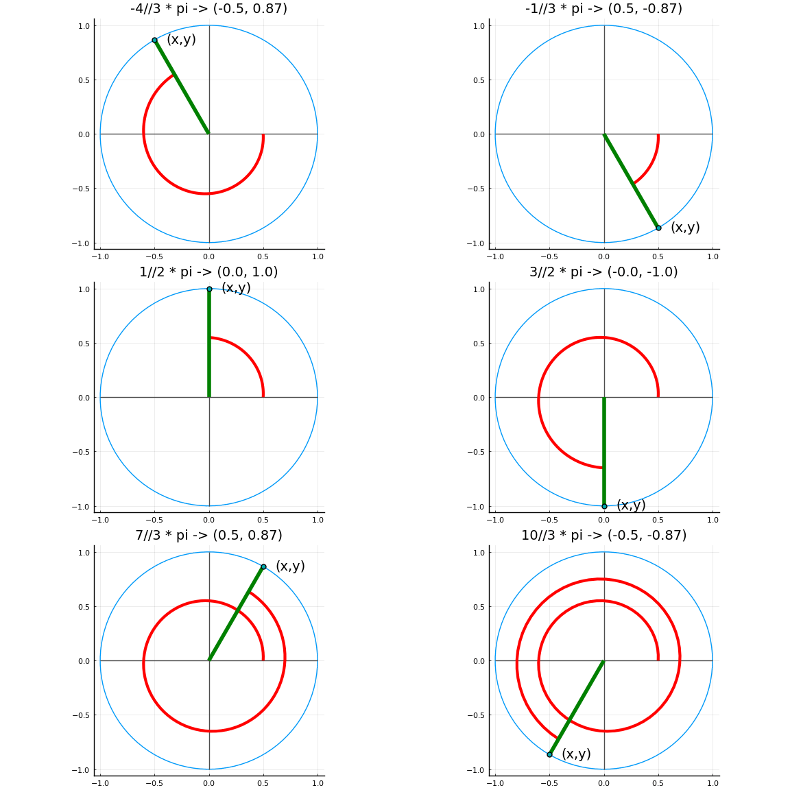
In the figure below, an angle in radians corresponds to a point on the unit circle, whose coordinates define the sine and cosine of the angle.

Example

julia> pi
π = 3.1415926535897...

julia> sin(0)
0.0

julia> sin(pi/6)
0.49999999999999994

julia> sin(pi/4)
0.7071067811865475

julia> cos(0)
1.0

julia> cos(pi/6)
0.8660254037844387

julia> cos(pi/3)
0.5000000000000001

All the functions provided above are single-argument functions, but atan can also accept two parameters to represent the traditional atan2 function.

atan(y)
atan(y, x)

Compute the arctangent of y or y/x, respectively.

Example

julia> theta = 3pi/4
2.356194490192345

julia> x,y = (cos(theta), sin(theta))
(-0.7071067811865475, 0.7071067811865476)

julia> atan(y/x)
-0.7853981633974484

julia> atan(y, x)
2.356194490192345

In addition, sinpi(x) and cospi(x) are used to compute sin(pi*x) and cos(pi*x) more accurately, respectively.

To compute trigonometric functions in degrees rather than radians, use d as a suffix. For example, sind(x) computes the sine of x, where x is an angle in degrees. The following is a complete list of trigonometric functions for angle variables:

sind   cosd   tand   cotd   secd   cscd
asind  acosd  atand  acotd  asecd  acscd

Example

julia> cos(56)
0.853220107722584

julia> cosd(56)
0.5591929034707468

Other Extensions