PyTorch Linear Regression
Linear regression is one of the most fundamental machine learning algorithms, used to predict a continuous value. It is a simple and common regression analysis method that aims to predict the output by fitting a linear function.
For a simple linear regression problem, the model can be expressed as:

- y is the predicted value (target value).
- \(x_1\), \(x_2\), \(x_n\) are input features.
- \(w_1\), \(w_2\), \(w_n\) are the weights to be learned (model parameters).
- b is the bias term.
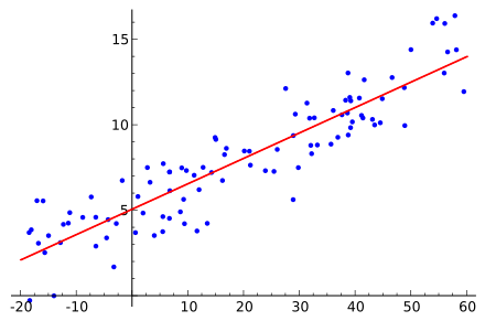
In PyTorch, a linear regression model can be implemented by inheritingnn.Modulethe class. We will use a simple example to explain in detail how to implement a linear regression model using PyTorch.
Data Preparation
We first prepare some fake data to train our linear regression model. Here, we can generate a dataset with a simple linear relationship, where each sample has two features \(x_1\), \(x_2\).
Example
import numpy as np
import matplotlib.pyplot as plt
# Random seed to ensure consistent results across runs
torch.manual_seed(42)
# Generate training data
X = torch.randn(100, 2) # 100 samples, each with 2 features
true_w = torch.tensor([2.0, 3.0]) # Assume true weights
true_b = 4.0 # Bias term
Y = X @ true_w + true_b + torch.randn(100) * 0.1 # Add some noise
# Print some data
print(X[:5])
print(Y[:5])
The output is as follows:
tensor([[ 1.9269,  1.4873],
        [ 0.9007, -2.1055],
        [ 0.6784, -1.2345],
        [-0.0431, -1.6047],
        [-0.7521,  1.6487]])
tensor([12.4460, -0.4663,  1.7666, -0.9357,  7.4781])
This code creates a linear dataset with noise.
- Input X is a 100x2 matrix, each sample has two features.
- Output Y is generated from the true weights and bias, with some random noise added.
- Using
torch.manual_seed(42)ensures consistent results across runs, making debugging and reproduction easier.
Defining the Linear Regression Model
We can define a simple linear regression model by inheritingnn.ModuleIn PyTorch, the core of linear regression is thenn.Linear()layer, which automatically handles the initialization of weights and biases.
Example
# Define linear regression model
class LinearRegressionModel(nn.Module):
def __init__(self):
super(LinearRegressionModel, self).__init__()
# Define a linear layer, input is 2 features, output is 1 prediction
self.linear = nn.Linear(2, 1) # Input dimension 2, output dimension 1
def forward(self, x):
return self.linear(x) # Forward propagation, return prediction result
# Create model instance
model = LinearRegressionModel()
Here,nn.Linear(2, 1)represents a linear layer, which has 2 input features and 1 output.forwardThe method defines how to perform forward propagation through this layer.
Note:
nn.Linearautomatically creates the weight matrix and bias vector, no need to define them manually.
Defining Loss Function and Optimizer
The common loss function for linear regression isMean Squared Error Loss (MSELoss), used to measure the difference between predicted and true values. PyTorch provides a ready-made MSELoss function.
We will useSGD (Stochastic Gradient Descent)orAdamoptimizer to minimize the loss function.
Example
criterion = nn.MSELoss()
# Optimizer (using SGD or Adam)
optimizer = torch.optim.SGD(model.parameters(), lr=0.01) # Learning rate set to 0.01
# You can also use Adam optimizer
# optimizer = torch.optim.Adam(model.parameters(), lr=0.01)
| Component | Description |
|---|---|
MSELoss |
Calculate the mean squared error between predicted and true values, formula: \(\frac{1}{n}\sum(y_{pred} - y_{true})^2\) |
SGD |
Use stochastic gradient descent to update parameters, learning rate controls the step size of each update |
Adam |
Adaptive learning rate optimizer, usually converges faster |
Training the Model
During training, we will perform the following steps:
- Use input data X for forward propagation to obtain predictions.
- Calculate the loss (difference between predicted and actual values).
- Use backpropagation to compute gradients.
- Update model parameters (weights and bias).
We will train the model for 1000 epochs and print the loss every 100 epochs.
Example
num_epochs = 1000 # Train for 1000 epochs
for epoch in range(num_epochs):
model.train() # Set model to training mode
# Forward propagation
predictions = model(X) # Model outputs predictions
loss = criterion(predictions.squeeze(), Y) # Calculate loss (note that predictions need to be squeezed to 1D)
# Backpropagation
optimizer.zero_grad() # Clear previous gradients
loss.backward() # Compute gradients
optimizer.step() # Update model parameters
# Print loss
if (epoch + 1) % 100 == 0:
print(f'Epoch [{epoch + 1}/1000], Loss: {loss.item():.4f}')
predictions.squeeze(): Squeeze the model output from a 2D tensor to 1D, because the target valueYis a one-dimensional array.optimizer.zero_grad(): Before each backpropagation, you need to clear the previous gradients, otherwise the gradients will accumulate.loss.backward(): Automatically computes the gradients of all trainable parameters.optimizer.step(): Updates the weights and bias based on the computed gradients.
Training mode vs evaluation mode:Calling in the training loop
model.train()is necessary. Although this example does not use Dropout or BatchNorm, developing this habit is important for complex models.
Evaluating the Model
After training, we can evaluate the model's performance by inspecting its weights and bias. We can also make predictions on new data and compare them with actual values.
Example
print(f'Predicted weight: {model.linear.weight.data.numpy()}')
print(f'Predicted bias: {model.linear.bias.data.numpy()}')
# Make predictions on new data
with torch.no_grad(): # No need to compute gradients during evaluation
predictions = model(X)
# Visualize predictions and actual values
plt.scatter(X[:, 0], Y, color='blue', label='True values')
plt.scatter(X[:, 0], predictions, color='red', label='Predictions')
plt.legend()
plt.show()
model.linear.weight.dataandmodel.linear.bias.data: These attributes store the model's weights and bias.torch.no_grad(): In evaluation mode, there is no need to compute gradients, which saves memory and improves inference speed.
Complete Example Code
Below is the complete code for all the above steps, integrated together and ready to run:
Example
import torch.nn as nn
import matplotlib.pyplot as plt
# 1. Prepare data
torch.manual_seed(42)
X = torch.randn(100, 2) # 100 samples, 2 features
true_w = torch.tensor([2.0, 3.0])
true_b = 4.0
Y = X @ true_w + true_b + torch.randn(100) * 0.1
# 2. Define model
class LinearRegressionModel(nn.Module):
def __init__(self):
super().__init__()
self.linear = nn.Linear(2, 1)
def forward(self, x):
return self.linear(x)
model = LinearRegressionModel()
# 3. Define loss function and optimizer
criterion = nn.MSELoss()
optimizer = torch.optim.SGD(model.parameters(), lr=0.01)
# 4. Train model
num_epochs = 1000
for epoch in range(num_epochs):
model.train()
predictions = model(X)
loss = criterion(predictions.squeeze(), Y)
optimizer.zero_grad()
loss.backward()
optimizer.step()
if (epoch + 1) % 100 == 0:
print(f'Epoch [{epoch + 1}/{num_epochs}], Loss: {loss.item():.4f}')
# 5. Evaluate model
print(f'\nTrained weights: {model.linear.weight.data.numpy()}')
print(f'Trained bias: {model.linear.bias.data.numpy()}')
print(f'True weights: {true_w.numpy()}')
print(f'True bias: {true_b}')
Analysis of Running Results
After running the code above, you will see output similar to the following:
Epoch [100/1000], Loss: 0.0654
Epoch [200/1000], Loss: 0.0398
Epoch [300/1000], Loss: 0.0243
Epoch [400/1000], Loss: 0.0148
Epoch [500/1000], Loss: 0.0090
Epoch [600/1000], Loss: 0.0055
Epoch [700/1000], Loss: 0.0033
Epoch [800/1000], Loss: 0.0020
Epoch [900/1000], Loss: 0.0012
Epoch [1000/1000], Loss: 0.0008

训练后的权重: [[2.0016 2.9973]]
训练后的偏置: [4.0015]
真实权重: [2. 3.]
真实偏置: 4.0
It can be seen that as the number of training epochs increases, the loss value continuously decreases. Eventually, the model's weights and bias are very close to the true values, indicating that the model has successfully learned the linear relationship of the data.
Extension: Using More Complex Optimizers
In addition to SGD, PyTorch provides many other optimizers. Below is an example using the Adam optimizer:
Example
optimizer = torch.optim.Adam(model.parameters(), lr=0.01)
# Train the model
for epoch in range(num_epochs):
model.train()
predictions = model(X)
loss = criterion(predictions.squeeze(), Y)
optimizer.zero_grad()
loss.backward()
optimizer.step()
if (epoch + 1) % 100 == 0:
print(f'Epoch [{epoch + 1}/{num_epochs}], Loss: {loss.item():.4f}')
| Optimizer | Features | Applicable Scenarios |
|---|---|---|
| SGD | Simple and straightforward, requires manual tuning of learning rate | Large datasets, classic scenarios |
| Adam | Adaptive learning rate, fast convergence | Most scenarios, recommended default choice |
| RMSprop | Suitable for recurrent neural networks | Sequence models such as RNN, LSTM |
Common Issues
Problem 1: Loss Value Not Decreasing
If the loss value does not decrease during training, possible reasons include:
- Learning rate too small, causing parameter updates to be too small.
- Learning rate too large, causing the optimal solution to be skipped.
- Issues with the data, such as feature value ranges differing too much.
Solution:
- Try adjusting the learning rate (start with 0.1, 0.01, 0.001).
- Standardize the input data.
- Check for outliers or missing values in the data.
Problem 2: Prediction Shape Mismatch
If a shape mismatch error occurs when calculating the loss, you may need to usesqueeze()orunsqueeze()Adjust the tensor shape.
Example
predictions = model(X)
print(f'Model output shape: {predictions.shape}') # Should be [100, 1]
# Squeeze to 1D
predictions = predictions.squeeze()
print(f'Shape after squeeze: {predictions.shape}') # Should be
# Compute loss
loss = criterion(predictions, Y)
Problem 3: How to Improve Model Accuracy
- Increase the number of training epochs.
- Adjust the learning rate.
- Use a more complex model structure (e.g., multi-layer neural network).
- Increase the amount of training data.