Jupyter Notebook Common Shortcuts and Practical Tips
Jupyter Notebook is the most popular interactive development environment in data science and machine learning. Mastering its shortcuts and tips can greatly improve daily development efficiency.
You can click the Help menu to view shortcuts:
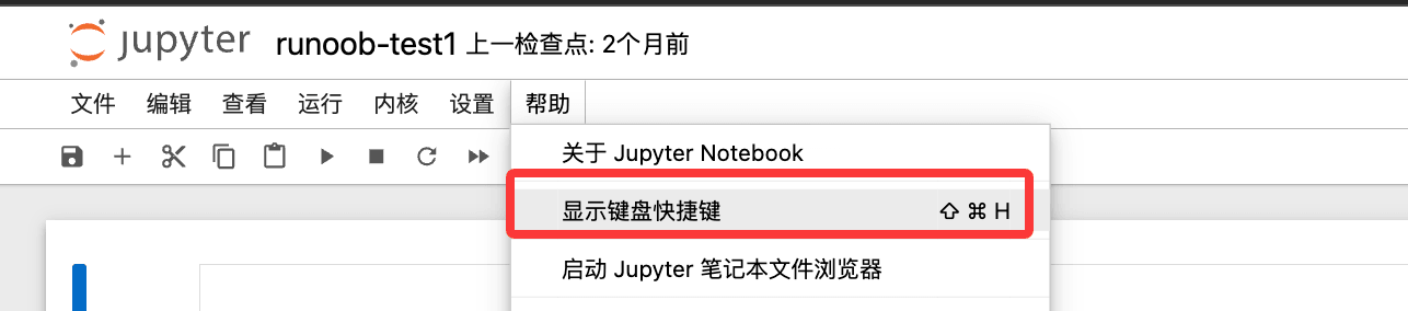
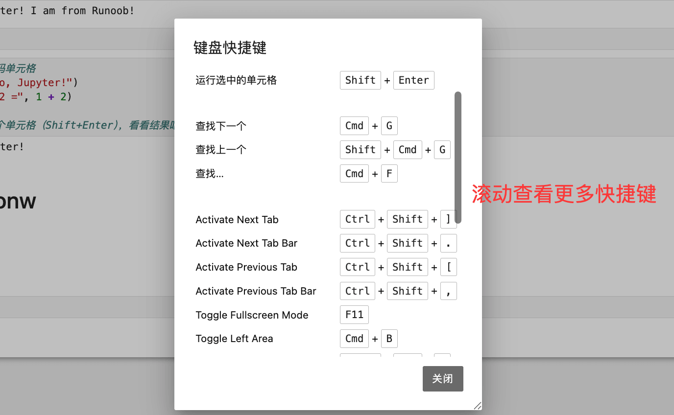
All shortcuts in this article are based onWindows/Linuxas the benchmark. Mac users should replace
CtrlwithCmd, and replaceAltwithOption。
Two operating modes
Jupyter Notebook has two modes,all shortcuts depend on the current mode, which is the key point most beginners overlook:
| Mode | Cell border color | How to enter | Function |
|---|---|---|---|
| Command Mode | Blue | pressEscor click the blank area on the left side of the Cell |
Manage Cells (add, delete, move, etc.) |
| Edit Mode | Green | pressEnteror double-click inside the Cell |
Write and modify code or text inside a Cell |
Quick memory aid:Green = can type and edit; Blue = can manage Cells. Before entering edit mode, first useEscto exit, then useEnterto enter. Developing this habit can avoid many accidental operations.
Shortcuts for running Cells (universal)
The following three shortcuts can be used in both modes. They are the most frequent operations, so be sure to memorize them:
| Shortcut | Function | Applicable scenario |
|---|---|---|
Shift + Enter |
Run the current Cell and automatically jump to the next Cell | Most common, execute code sequentially downward |
Ctrl + Enter |
Run the current Cell and stay on the current Cell | Use when repeatedly testing the same code |
Alt + Enter |
Run the current Cell and insert a new Cell below | Use when adding code blocks downward while running |
Command mode shortcuts (blue border)
pressEscAfter entering command mode, you can use the following shortcuts:
1. Insertion and deletion of Cells
| Shortcut | Function |
|---|---|
A |
At the current CellAboveInsert a new Cell (Above) |
B |
At the current CellBelowInsert a new Cell (Below) |
D, D(Press D twice) |
Delete the current Cell |
Z |
Undo delete (restore the just-deleted Cell) |
X |
Cut the current Cell |
C |
Copy the current Cell |
V |
Paste a Cell below the current Cell |
Shift + V |
Paste a Cell above the current Cell |
2. Cell type switching
Cells in Jupyter have three types, which can be switched at any time:
| Shortcut | Switch to | Purpose |
|---|---|---|
Y |
Code | Write and run Python code |
M |
Markdown (markup language) | Write formatted documentation, headings, descriptions |
R |
Raw (raw text) | Output text as is, without executing or rendering |
1 ~ 6 |
Markdown heading levels H1 ~ H6 | Quickly set the Cell to the corresponding heading level (automatically switches to Markdown mode) |
3. Selecting and merging Cells
| Shortcut | Function |
|---|---|
↑ / K |
Select the Cell above |
↓ / J |
Select the Cell below |
Shift + ↑ / Shift + K |
Select multiple Cells upward (continuously) |
Shift + ↓ / Shift + J |
Select multiple Cells downward (continuously) |
Shift + M |
Merge the selected Cells into one |
4. Output and display control
| Shortcut | Function |
|---|---|
O |
Collapse/expand the output of the current Cell |
Shift + O |
Toggle scrolling mode for the current Cell's output area (use when output content is very long) |
L |
Show/hide line numbers for the current Cell |
F |
Find and replace text in the Cell |
5. Kernel and interface operations
| Shortcut | Function |
|---|---|
I, I(Press I twice) |
Interrupt the currently running Cell (equivalent to Ctrl+C) |
0, 0(Press 0 twice) |
Restart the kernel (this will clear all executed variables,use with caution) |
H |
Open the shortcut help panel (shows all available shortcuts) |
P |
Open the command palette to search all Jupyter functions |
Space |
Scroll down the page |
Shift + Space |
Scroll up the page |
S / Ctrl + S |
Save Notebook |
Edit mode shortcuts (green border)
pressEnterAfter entering edit mode, you can use the following shortcuts to operate inside a Cell:
1. Code editing
| Shortcut | Function |
|---|---|
Tab |
Code auto-completion (type part of a function/variable name then press Tab to complete) |
Shift + Tab |
View the parameter description of the function at the cursor (pops up a documentation tooltip; press once for a brief summary, press twice for the full documentation) |
Ctrl + / |
Comment/uncomment the current line or selected multiple lines of code |
Ctrl + D |
Delete the entire current line |
Ctrl + Shift + - |
Split the current Cell into two Cells at the cursor |
Ctrl + Z |
Undo (restore the previous edit) |
Ctrl + Y |
Redo (undo the undo) |
Ctrl + A |
Select all contents in the current Cell |
Ctrl + Home |
Jump to the very beginning of the Cell content |
Ctrl + End |
Jump to the very end of the Cell content |
Ctrl + ← / Ctrl + → |
Jump cursor by word (quickly move to the previous/next word) |
2. Return from edit mode to command mode
| Shortcut | Function |
|---|---|
Esc |
Exit edit mode, return to command mode (Cell border turns blue) |
Ctrl + M |
Same as Esc, exit edit mode |
Magic Commands
Magic commands are special built-in Jupyter directives that start with%(single line) or%%(entire Cell), used to accomplish common tasks such as timing, debugging, file operations, etc.They can be used without installing any libraries.。
1. Code timing
Example
%timeit [x**2 for x in range(1000)]
# Example output: 98.3 µs ± 1.2 µs per loop (mean ± std. dev. of 7 runs, 10000 loops each)
# %%time: times the code of the entire Cell once (suitable for testing complete processes that take a long time)
%%time
import time
data = [x**2 for x in range(100000)]
time.sleep(1)
# Example output:
# CPU times: user 45.2 ms, sys: 8.1 ms, total: 53.3 ms
# Wall time: 1.05 s
2. Inline display of charts
Example
# Usually placed in the first Cell of the Notebook; only needs to be executed once for the entire Notebook
%matplotlib inline
import matplotlib.pyplot as plt
import numpy as np
x = np.linspace(0, 2 * np.pi, 100)
plt.plot(x, np.sin(x))
plt.title('sine wave')
plt.show()
# %matplotlib notebook: enables interactive charts that can be zoomed and panned (but cannot be used together with inline)
# %matplotlib notebook
3. Viewing and managing variables
Example
%who
# Example output: data plt x
# %whos: more detailed than %who, also displays the type and value of variables
%whos
# Example output:
# Variable Type Data/Info
# ----------------------------
# x ndarray 100: [0. 0.06 ... 6.28]
# data list n=100000
# %reset: clears all variables (shows a confirmation prompt; suitable when restarting calculations)
%reset
# %reset -f: forcefully clears all variables without a confirmation prompt (-f means force)
%reset -f
4. File and path operations
Example
%pwd
# Example output: '/home/user/notebooks'
# %ls: lists all files in the current directory (Windows users may need to use %ls or directly use !dir)
%ls
# Example output: data.csv model.py notebook.ipynb
# %%writefile: writes the content of the entire Cell to a specified file (commonly used to quickly create script files)
%%writefile hello.py
def greet(name):
print(f"Hello, {name}!")
greet("World")
# After execution, a hello.py file is generated in the current directory, containing the code in the Cell
# %run: runs an external Python script file and imports its variables into the current namespace
%run hello.py
# Output: Hello, world!
# %load: loads the content of an external script file into the current Cell (does not automatically execute; only loads the code)
%load hello.py
5. Executing system commands
Example
!pip install pandas # Install Python packages
!pip list # View the list of installed packages
!python --version # View the Python version
# You can also save the command output as a Python variable
files = !ls -1 # Execute the ls command and assign the result to the variable files
print(files) # files is a list, where each file name is an element
6. Viewing history and debugging
Example
%history
# Adding -n displays line numbers; adding -l 5 shows only the most recent 5 entries
%history -n -l 5
# %debug: after code reports an error, running %debug in the next Cell enters interactive debugging mode
# In debug mode, you can enter variable names to view values, and enter q to exit debugging
# For example, after running a piece of code that caused an error:
%debug
7. Rendering special content
Example
%%html
<h3 style="color: steelblue;">This is an HTML heading</h3>
<p style="font-size: 16px;">HTML content can be rendered directly in the Notebook.</p>
# %%latex: renders the Cell content as a LaTeX formula (often used for writing mathematical formulas)
%%latex
$$E = mc^2$$
$$\int_0^\infty e^{-x^2} dx = \frac{\sqrt{\pi}}{2}$$
View running progress in real time
When processing large amounts of data or running long loops, it is very important to view progress in real time. Below are several commonly used progress display solutions.
1. tqdm progress bar (recommended)
tqdm is the most commonly used progress bar library, supporting loops, Pandas, and various Jupyter scenarios. Installation command:
pip install tqdm
Example
import time
# Basic usage: wrap an iterable object in tqdm() to automatically display a progress bar
for i in tqdm(range(100)):
time.sleep(0.05) # Simulate a time-consuming operation
# Output: displays progress bar, percentage completed, elapsed time, estimated remaining time
# Use with enumerate
data = list(range(50))
for i, item in enumerate(tqdm(data, desc="Processing data")):
# The desc parameter sets the label text on the left side of the progress bar
time.sleep(0.05)
# Manually control progress (suitable for scenarios where the total is uncertain)
with tqdm(total=100, desc="Download progress") as pbar:
for chunk in range(10):
time.sleep(0.1)
pbar.update(10) # Update progress by 10 units each time
pbar.set_postfix({"chunk": chunk}) # Display additional information on the right side of the progress bar
Example
import pandas as pd
from tqdm.notebook import tqdm
tqdm.pandas() # Enable Pandas integration; only needs to be executed once
df = pd.DataFrame({'value': range(1000)})
# Use progress_apply instead of ordinary apply to automatically display progress
result = df['value'].progress_apply(lambda x: x ** 2)
2. display + clear_output dynamic refresh output
When you don't want to install tqdm, you can use IPython's built-inclear_outputto achieve dynamic refresh effects:
Example
import time
total = 50
for i in range(total):
time.sleep(0.1)
# clear_output(wait=True): clears the previous output; wait=True means wait until new content is available before clearing,
# to avoid flickering. Note: this clears all output of the current Cell
clear_output(wait=True)
# Manually draw a simple text progress bar
done = int((i + 1) / total * 30) # Calculate the number of completed cells (30 cells in total)
bar = '█' * done + '░' * (30 - done) # █ means completed, ░ means not completed
pct = (i + 1) / total * 100
print(f"Progress: [{bar}] {pct:.1f}% ({i+1}/{total})")
print("✅ All done!")
3. Real-time chart drawing progress
In scenarios such as model training, you can dynamically update charts at intervals to observe metric trends in real time:
Example
import matplotlib.pyplot as plt
from IPython.display import clear_output, display
import numpy as np
import time
losses = [] # Store the loss value of each step to simulate the training process
for step in range(50):
# Simulate training: generate a gradually decreasing loss value
loss = 1 / (step + 1) + np.random.uniform(0, 0.05)
losses.append(loss)
# Update the chart every 5 steps to avoid refreshing too frequently
if (step + 1) % 5 == 0:
clear_output(wait=True)
fig, ax = plt.subplots(figsize=(8, 4))
ax.plot(losses, color='steelblue', linewidth=2)
ax.set_title(f'Training progress (Step {step + 1}/50)')
ax.set_xlabel('Step')
ax.set_ylabel('Loss')
ax.grid(True, alpha=0.3)
plt.tight_layout()
plt.show() # Call show after clear_output, and the chart will refresh in the same position
time.sleep(0.1)
print("Training complete! Final Loss:", f"{losses[-1]:.4f}")
Tips for viewing documentation and code
1. Quickly view function documentation
Example
import numpy as np
np.array?
# This pops up the parameter description and functional description of np.array
# Method 2: add ?? after the function name to pop up the complete documentation, including source code (if the source is available)
np.array??
# Method 3: press Shift + Tab inside the function parentheses
# For example, after typing np.linspace( (inside the parentheses) press Shift + Tab to pop up parameter hints
# Press Shift + Tab twice to display more complete documentation
# Method 4: use the help() function (output is more complete, but displayed in the output area rather than a popup)
help(np.array)
2. Use display to show multiple output results
By default, Jupyter only displays the value of the last expression in each Cell. Throughdisplay()you can output multiple results in one Cell:
Example
from IPython.display import display
df1 = pd.DataFrame({'A': [1, 2, 3], 'B': [4, 5, 6]})
df2 = pd.DataFrame({'X': [7, 8, 9], 'Y': [10, 11, 12]})
# Without display, only the last DataFrame is displayed
# df1 # will not be displayed
# df2 # Only this one will display
# Using display() can display multiple tables at once, with nice formatting
display(df1)
display(df2)
Example
from IPython.core.interactiveshell import InteractiveShell
InteractiveShell.ast_node_interactivity = "all" # Default is "last_expr"; after changing to "all"
# Every expression in the Cell will automatically output its result
1 + 1 # Outputs 2
2 + 2 # Outputs 4 (by default this line won't output)
"hello" # Outputs 'hello'
3. Suppress unwanted output
Example
import numpy as np
# Problem: plt.plot() will output an extra object description while displaying the chart, like:
# [<matplotlib.lines.Line2D object at 0x7f3b1234>]
# Solution: Add a semicolon (;) at the end of the statement to suppress the output of the last expression without affecting the chart display
plt.plot(np.sin(np.linspace(0, 2*np.pi, 100)));
# After adding the semicolon, the chart displays normally, but the extra object description won't appear
Other practical tips
1. View intermediate values of variables (without interrupting code execution)
Example
# While assigning the intermediate result to a variable, wrap the entire line in parentheses to make it output
import numpy as np
# Normal way (can't see the value of result)
result = np.array([1, 2, 3]) * 2
# Parenthesized way (prints the value of result while assigning)
(result := np.array([1, 2, 3]) * 2) # Python 3.8+ walrus operator approach
# Output: array([2, 4, 6])
# Or simpler: just write the variable name on a new line after the assignment
result = np.array([1, 2, 3]) * 2
result # Jupyter will automatically display the value of the last expression
2. Reference the previous output result
Example
# _ : Output result of the previous Cell
# __ : Output result of the Cell before the previous one
# _3 : Output result of the 3rd Cell (Out
# For example:
1 + 1
# Out[1]: 2
_ # Reference the previous output, value is 2
# Out[2]: 2
_ * 10 # Use the previous output to continue calculating
# Out[3]: 20
_3 + 5 # Reference the result 20 of Out
# Out[4]: 25
3. Display rich text content in Notebook
Example
# Render Markdown formatted text
display(Markdown("## This is a heading\n\n**bold text**, *italic text*, `code`"))
# Render HTML
display(HTML("<span style='color:red; font-size:20px'>Big red text</span>"))
# Display a network image (pass the image URL)
display(Image(url="https://www.example.com/images/example-logo.png", width=200))
# Display a local image (pass the local file path)
# display(Image(filename="./chart.png"))
4. Add timing annotations to Cells (automatically display elapsed time in output)
Example
# pip install jupyter-contrib-nbextensions
# Simple solution: use a decorator or context manager to encapsulate the timing logic, usable in any code block
import time
from contextlib import contextmanager
@contextmanager
def timer(label="Elapsed time"):
start = time.time()
try:
yield
finally:
elapsed = time.time() - start
print(f"⏱ {label}: {elapsed:.3f} seconds")
# Usage: wrap any code block with with timer():, and the elapsed time will be printed automatically after execution
with timer("Data processing"):
data = [x ** 2 for x in range(1000000)]
# Output: ⏱ Data processing: 0.087 seconds
5. Quickly view all shortcuts for the current Notebook
In command mode (blue border), pressH, or via the menuHelp → Keyboard Shortcuts, to open the complete shortcut help panel, and check all available operations at any time.
Common shortcut keys quick reference table
| Operation | Shortcut | Mode |
|---|---|---|
| Run Cell and jump to the next | Shift + Enter |
General |
| Run Cell and stay in place | Ctrl + Enter |
General |
| Run Cell and create new below | Alt + Enter |
General |
| Enter edit mode | Enter |
Command mode |
| Exit edit mode | Esc |
Edit mode |
| Insert Cell above | A |
Command mode |
| Insert Cell below | B |
Command mode |
| Delete Cell | D, D |
Command mode |
| Undo Cell deletion | Z |
Command mode |
| Switch to Code Cell | Y |
Command mode |
| Switch to Markdown Cell | M |
Command mode |
| Merge multiple selected Cells | Shift + M |
Command mode |
| Interrupt kernel (stop running) | I, I |
Command mode |
| Restart kernel | 0, 0 |
Command mode |
| Show shortcut help | H |
Command mode |
| Code auto-completion | Tab |
Edit mode |
| View function parameters/documentation | Shift + Tab |
Edit mode |
| Comment/uncomment | Ctrl + / |
Edit mode |
| Split Cell at cursor | Ctrl + Shift + - |
Edit mode |
| Save Notebook | S / Ctrl + S |
Command mode / Edit mode |