Tree structure
A tree is anon-linearA data structure that simulates the branching hierarchy of trees in nature. Unlike linear structures such as arrays and linked lists, where elements are arranged one after another, the data elements in a tree (callednode) there is a clear one-to-many hierarchical relationship among them.
Tree structureJust like a real tree:
- root node: the root part of the tree, the only node without a parent node
- child node: nodes that branch out from a node
- leaf node: a node with no children, like a leaf
- path: the route from one node to another node
- depth: the path length from the root node to this node
- height: the path length from this node to the farthest leaf node
Life analogy:
- family tree: grandparents → parents → children → grandchildren
- organizational structure: CEO → director → manager → employee
- file system: root directory → subdirectory → file
- book classification: general category → subcategory → specific book
| structure type | search efficiency | insertion efficiency | deletion efficiency | ordering |
|---|---|---|---|---|
| array | O(n) | O(n) | O(n) | None |
| Linked list | O(n) | O(1) | O(1) | None |
| Hash table | O(1) | O(1) | O(1) | None |
| binary search tree | O(log n) | O(log n) | O(log n) | Yes |
Basic Terms
Before going deeper, let's first get familiar with the basic terminology of trees:
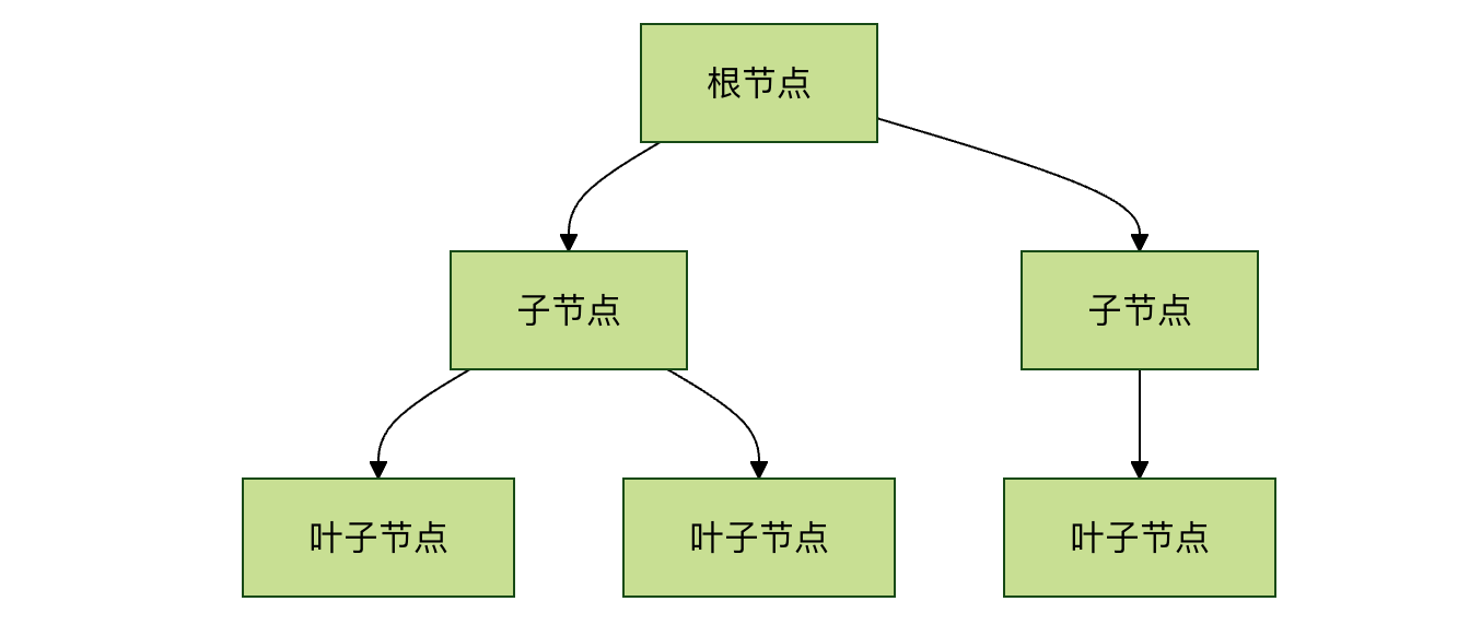
- Node: every element in a tree. It contains the stored data and links to its child nodes.
- Root node: the node at the top of the tree, the starting point of the entire tree. A tree has exactly one root node.
- Parent node and child node (Parent & Child): If a node A is connected to a node B below it, then A is B'sparent node, B is A'schild node. A parent node can have multiple child nodes.
- Sibling nodes (Siblings): nodes that share the same parent node are siblings.
- Leaf node (Leaf): a node with no child nodes, also called a terminal node.
- Edge: the line connecting two nodes, representing the relationship between them.
- Path: the sequence of nodes passed through from the root node to a specific node.
- Height: on the longest path from a node to its farthest leaf nodenumber of edges. The height of the tree is the height of the root node.
- Depth: on the path from the root node to a specific nodenumber of edges. The depth of the root node is 0.
- Level: all nodes with the same depth belong to the same level. The root node is at level 0.
Basic properties of trees
- unique path: there is exactly one path between any two nodes in a tree.
- N nodes, N-1 edges: a tree with N nodes has a total of N-1 edges.
- acyclic: there are no cycles in a tree (i.e., starting from a node and following edges, you cannot return to that node).
Why do we need trees? — Advantages and Applications of Trees
You may ask: with arrays and linked lists, why do we still need trees? The answer lies in efficiency.
- array: fast lookup (via index), but slow insertion and deletion (requires moving many elements).
- Linked list: fast insertion and deletion, but slow lookup (requires traversing from the beginning).
- Trees (especially binary search trees): While keeping data ordered, it can provide much faster search speed than linked lists, and more efficient insertion/deletion operations than arrays.
Practical application scenarios:
- file system: folders and files in computers are organized in the form of a tree.
- database index: B-tree and B+ tree are core data structures for efficient queries in databases.
- organization chart: the hierarchical management of a company or department.
- decision tree: classification models in artificial intelligence and machine learning.
- HTML DOM: the Document Object Model of a web page is a tree.
Binary tree: the most important member of the tree family
A Binary Tree is a tree in which each node has at most two child nodes. These two child nodes are usually calledleft child nodeandright child node, it is the foundation of many powerful tree structures (such as binary search trees, heaps, and AVL trees).
The basic structure is as follows:
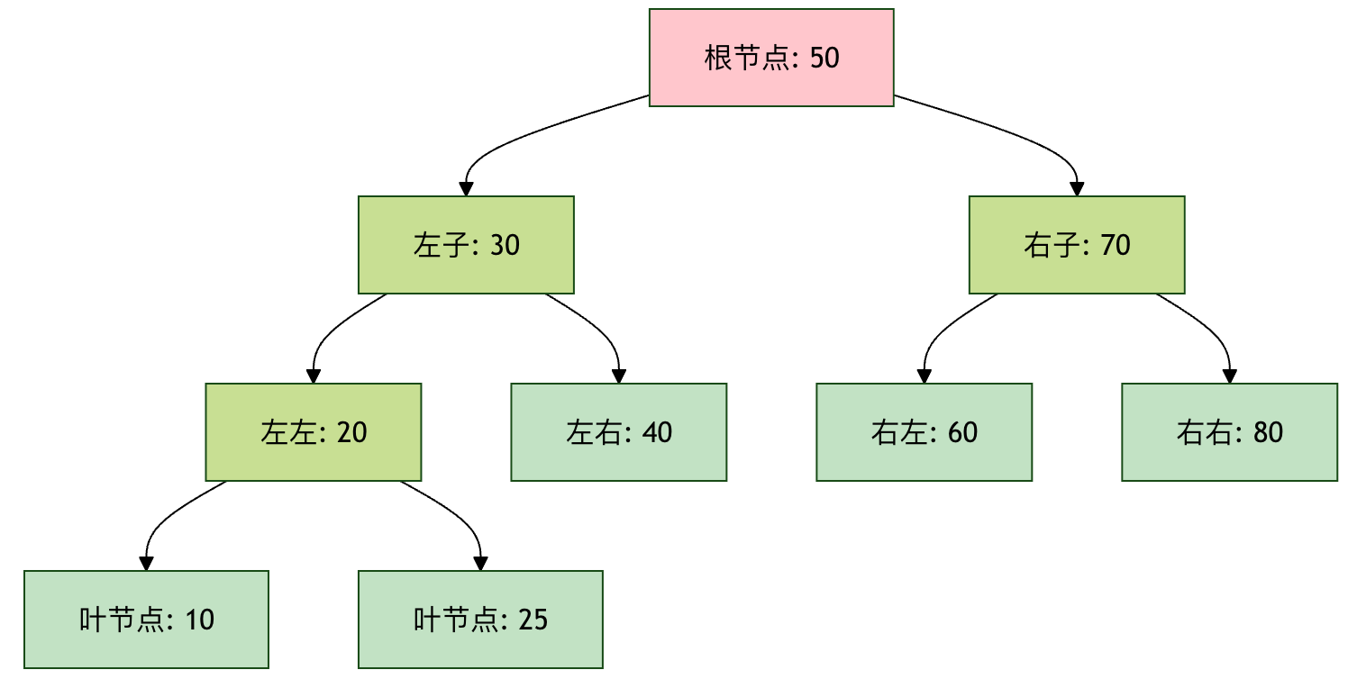
Basic terms for binary trees
| Term | definition | Life Analogy |
|---|---|---|
| node | the basic unit containing data and pointers | A person in the family |
| root node | The top node of a tree | Ancestor in the family |
| parent node | A node with child nodes | parents |
| child node | the node pointed to by its parent node | children |
| sibling node | child nodes of the same parent | siblings |
| leaf node | a node with no children | a person in the family with no children |
| depth | the number of edges from the root to this node | number of generations |
| height | the number of edges from this node to the farthest leaf node | the number of generations the family continues |
binary tree type
| Type | Features | Time complexity | application scenarios |
|---|---|---|---|
| ordinary binary tree | each node has at most 2 child nodes | O(n) | expression tree |
| full binary tree | each node has either 0 or 2 child nodes | O(n) | Huffman coding |
| complete binary tree | all levels except the last are full | O(n) | heap implementation |
| binary search tree | left < root < right | Average O(log n) | Searching, sorting |
| balanced binary tree | the height difference between the left and right subtrees is ≤ 1 | O(log n) | database index |
| red-black tree | Colored balanced tree | O(log n) | Linux kernel |
Binary search tree operations
| Operation | Description | Time complexity |
|---|---|---|
| Search | Find a node by value | average O(log n), worst O(n) |
| Insert | insert new node | average O(log n), worst O(n) |
| Delete | Delete the specified node | average O(log n), worst O(n) |
| traversal | Visit all nodes | O(n) |
Binary tree traversal
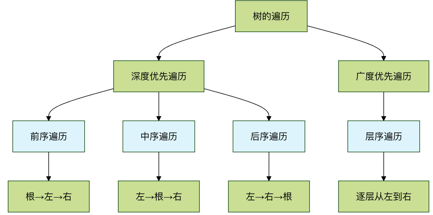
Traversal means visiting every node in the tree according to some rule, and each node is visited only once. This is the foundation of tree-related algorithms. There are mainly four ways:
Pre-order traversal:Root -> Left -> Right
- First visit the root node, then recursively preorder traverse the left subtree, and finally recursively preorder traverse the right subtree.
- Application: Copy a tree, get prefix expression.
In-order traversal:Left -> Root -> Right
- First recursively inorder traverse the left subtree, then visit the root node, and finally recursively inorder traverse the right subtree.
- Application: inbinary search treeAmong them, in-order traversal willascending orderOutput all values.
Post-order traversal:Left -> Right -> Root
- First recursively postorder traverse the left subtree, then recursively postorder traverse the right subtree, and finally visit the root node.
- Application: Delete a tree, calculate directory size.
Level-order traversal:By level, from left to right
- Starting from the root node, visit nodes level by level.
- Application: process data by levels (e.g., printing an organization chart).It is usually implemented with the help of a queue (Queue).。
Example: For the binary tree below, the traversal results are as follows:
        1
       / \
      2   3
     / \   \
    4   5   6
- preorder:1, 2, 4, 5, 3, 6
- inorder:4, 2, 5, 1, 3, 6
- postorder:4, 5, 2, 6, 3, 1
- level order:1, 2, 3, 4, 5, 6
Practice: Implement a Binary Tree in Python
Enough theory, let's write some code! We will implement a simple binary tree node class and complete insertion and traversal operations.
Step 1: Define the node class
Each node needs to store data and point to its left and right child nodes.
Example
"""Binary tree node class"""
def __init__(self, value):
self.value = value # Data stored in the node
self.left = None # Points to left child node
self.right = None # Points to right child node
def __str__(self):
"""Convenient for printing node information"""
return f"Node({self.value})"
Step 2: Build an example tree
Let's manually build the tree from the earlier example diagram.
Example
root = TreeNode(1)
node2 = TreeNode(2)
node3 = TreeNode(3)
node4 = TreeNode(4)
node5 = TreeNode(5)
node6 = TreeNode(6)
# Build connection relationships (Links)
root.left = node2
root.right = node3
node2.left = node4
node2.right = node5
node3.right = node6
print(f"Root node: {root}")
print(f"Root node's left child: {root.left}")
print(f"Root node's right child: {root.right}")
Step 3: Implement traversal algorithms (recursive version)
Recursion is the most intuitive way to implement tree traversal.
Example
"""Preorder traversal: root -> left -> right"""
if node is None:
return
print(node.value, end=' ') # 1. Visit root node
preorder_traversal(node.left) # 2. Traverse left subtree
preorder_traversal(node.right) # 3. Traverse right subtree
def inorder_traversal(node):
"""Inorder traversal: left -> root -> right"""
if node is None:
return
inorder_traversal(node.left) # 1. Traverse left subtree
print(node.value, end=' ') # 2. Visit root node
inorder_traversal(node.right) # 3. Traverse right subtree
def postorder_traversal(node):
"""Postorder traversal: left -> right -> root"""
if node is None:
return
postorder_traversal(node.left) # 1. Traverse left subtree
postorder_traversal(node.right) # 2. Traverse right subtree
print(node.value, end=' ') # 3. Visit root node
print("\n--- Traversal Demo ---")
print("Preorder traversal result:", end=' ')
preorder_traversal(root) # Output: 1 2 4 5 3 6
print("\nInorder traversal result:", end=' ')
inorder_traversal(root) # Output: 4 2 5 1 3 6
print("\nPostorder traversal result:", end=' ')
postorder_traversal(root) # Output: 4 5 2 6 3 1
Step 4: Implement level-order traversal (using a queue)
Level-order traversal needs to use the "first-in, first-out" property of a queue.
Example
def level_order_traversal(root):
"""Level-order traversal: using a queue"""
if root is None:
return
queue = deque([root]) # Initialize queue and enqueue root node
while queue:
current_node = queue.popleft() # 1. Pop node from the left of the queue
print(current_node.value, end=' ') # 2. Visit this node
# 3. Add this node's child nodes (if any) to the right side of the queue in order
if current_node.left:
queue.append(current_node.left)
if current_node.right:
queue.append(current_node.right)
print("\nLevel-order traversal result:", end=' ')
level_order_traversal(root) # Output: 1 2 3 4 5 6
Practice and Challenge
Congratulations on completing the basic learning! To truly master trees, hands-on practice is essential.
Exercise 1: Calculate the height of the tree
Write a functiontree_height(node), takes a tree's root node and returns the height of the tree (the height of an empty tree is -1 or 0, by convention; in this example we define it as the number of edges).
Hint: tree height = 1 + max(left subtree height, right subtree height). This is a classic recursive problem.
Exercise 2: Search for a value in a binary tree
Write a functionsearch_in_tree(node, target_value), in the given binary tree, search whether there is a value equal totarget_valuethe node. If found, returnTrue, otherwise returnFalse。
Hint: any traversal method can be used, and compare the value of each node when visiting it.
Challenge: Binary Search Tree (BST)
This is a classic variant of the binary tree. In a binary search tree, for any node:
- itsleft subtreethe values of all nodes in<The value of that node.
- itsright subtreethe values of all nodes in>The value of that node.
Your challenge is:
- Implementation
insert_into_bst(root, value)function, insert a value into the correct position in the binary search tree. - Implementation
search_in_bst(root, value)function, which uses the properties of BST for efficient search (average time complexity O(log N)).