Sklearn Machine Learning Models
Machine learning models are core tools for automated data analysis, pattern recognition, and prediction.
Depending on the task type, machine learning models can generally be divided into:
- Classification Models:Predict discrete categories
- Regression Models:Predict continuous values
- Clustering Models:Automatically group data
This chapter will introduce these common machine learning models in detail and explain how to evaluate and optimize them.
1. Classification Models
Classification is one of the most common problems in machine learning, with the goal of mapping input data to discrete class labels.
Common classification models include:
- Logistic Regression
- K-Nearest Neighbors (KNN)
- Support Vector Machine (SVM)
- Decision Tree
- Random Forest
Logistic Regression
Although logistic regression has "regression" in its name, it is essentiallya probabilistic classification model, often used for binary classification problems.
Its core idea is:
- First perform a linear weighted sum
- Then use the Sigmoid function to map the result to between 0 and 1 as a probability
It can be expressed as:
The core formula of logistic regression is:

scikit-learn implementation:
Example
from sklearn.model_selection import train_test_split
# Assume X is the feature matrix, y is the label
X_train, X_test, y_train, y_test = train_test_split(X, y, test_size=0.3, random_state=42)
model = LogisticRegression()
model.fit(X_train, y_train)
# Predict
y_pred = model.predict(X_test)
K-Nearest Neighbors (KNN)
K-Nearest Neighbors (KNN) is an instance-based learning method. During prediction, it calculates the distances between the sample to be predicted and all samples in the training set, selects the K nearest neighbors, and makes predictions based on the labels of those neighbors.
Main parameters:
- K: Number of neighbors to select.
- Distance metric: Euclidean distance is commonly used; Manhattan distance, Minkowski distance, etc. can also be used.
scikit-learn implementation:
Example
from sklearn.model_selection import train_test_split
# Assume X is the feature matrix, y is the label
X_train, X_test, y_train, y_test = train_test_split(X, y, test_size=0.3, random_state=42)
model = KNeighborsClassifier(n_neighbors=3)
model.fit(X_train, y_train)
# Predict
y_pred = model.predict(X_test)
Support Vector Machine (SVM)
Support Vector Machine is a powerful classification model, especially suitable for high-dimensional data.
The basic idea of SVM is to find a hyperplane that maximizes the margin between sample points of different classes. For non-linearly separable data, SVM uses the kernel trick to map the data into a higher-dimensional space and find a separating hyperplane.
Kernel functions:
- Linear kernel: Suitable for linearly separable data.
- Gaussian Radial Basis Function kernel (RBF): Suitable for non-linear data.
- Polynomial kernel: Suitable for data with polynomial relationships.
scikit-learn implementation:
Example
from sklearn.model_selection import train_test_split
# Assume X is the feature matrix, y is the label
X_train, X_test, y_train, y_test = train_test_split(X, y, test_size=0.3, random_state=42)
model = SVC(kernel='linear') # Use linear kernel
model.fit(X_train, y_train)
# Predict
y_pred = model.predict(X_test)
Decision Tree & Random Forest
Decision Tree is a tree-structured classification model that splits data and ultimately divides it into different classes. Random Forest, on the other hand, builds multiple decision trees and determines the final prediction through voting or averaging.
Decision TreeIt splits data by selecting optimal features. The selection criteria are usuallyinformation gainorGini coefficient。
Random ForestIt reduces overfitting and improves model accuracy through the ensemble of multiple decision trees. It increases model diversity by introducing randomness (e.g., randomly selecting features, randomly selecting data subsets).
scikit-learn implementation:
Example
from sklearn.ensemble import RandomForestClassifier
from sklearn.model_selection import train_test_split
# Assume X is the feature matrix, y is the label
X_train, X_test, y_train, y_test = train_test_split(X, y, test_size=0.3, random_state=42)
# Decision tree
dt_model = DecisionTreeClassifier()
dt_model.fit(X_train, y_train)
# Random forest
rf_model = RandomForestClassifier(n_estimators=100)
rf_model.fit(X_train, y_train)
# Predict
dt_pred = dt_model.predict(X_test)
rf_pred = rf_model.predict(X_test)
2. Regression Models
The goal of regression problems is to predict a continuous output variable. Common regression models include Linear Regression, Ridge Regression, and Lasso Regression.
Linear Regression
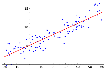
Linear Regression predicts the target variable by fitting a straight line. Its core assumption is that there is a linear relationship between the features and the target variable.
For a simple linear regression problem, the model can be expressed as:

- y is the predicted value (target value).
- x1,x2,xnis the input feature.
- w1,w2,wnare the weights to be learned (model parameters).
- b is the bias term.
scikit-learn implementation:
Example
from sklearn.model_selection import train_test_split
# Assume X is the feature matrix, y is the target variable
X_train, X_test, y_train, y_test = train_test_split(X, y, test_size=0.3, random_state=42)
model = LinearRegression()
model.fit(X_train, y_train)
# Predict
y_pred = model.predict(X_test)
Ridge Regression
Ridge Regression is a variant of Linear Regression that usesL2 regularizationto constrain the complexity of the model and avoid overfitting.
By penalizing the magnitude of regression coefficients, Ridge Regression can better handle multicollinearity problems.
Example
model = Ridge(alpha=1.0) Example
model.fit(X_train, y_train)
# alpha is the regularization parameter
y_pred = model.predict(X_test)
Lasso Regression
Lasso RegressionLasso Regression is also a form of Linear Regression; it usesL1 regularization
to penalize the regression coefficients.
Example
model = Lasso(alpha=0.1) scikit-learn implementation:
model.fit(X_train, y_train)
Example
y_pred = model.predict(X_test)
3. Clustering Models
# Predict
K-Means
Clustering is an unsupervised learning method whose goal is to divide objects in a dataset into different groups (or clusters), making objects within the same cluster as similar as possible, and objects in different clusters as different as possible.
K-Means
Example
scikit-learn implementation:
model = KMeans(n_clusters=3)
model.fit(X)
Example
labels = model.predict(X)
DBSCAN (Density-Based Clustering)
# Get cluster labels
DBSCAN (Density-Based Clustering)
Example
scikit-learn implementation:
model = DBSCAN(eps=0.5, min_samples=5)
model.fit(X)
# Get cluster labels
labels = model.labels_
Hierarchical Clustering
Hierarchical clustering is a method of clustering by recursively merging or splitting clusters. Commonly used hierarchical clustering methods includeAgglomerative clustering(Agglomerative) andDivisive clustering(Divisive)。
scikit-learn Implementation:
Example
# Assume X is the feature matrix
model = AgglomerativeClustering(n_clusters=3)
labels = model.fit_predict(X)
4. Model Evaluation and Selection
In machine learning, after model training is completed, it is necessary to evaluate the model's generalization ability through reasonable evaluation methods and select the model with the best performance.
Common evaluation methods include:
- Classification metrics evaluation
- Cross-validation
- Hyperparameter tuning
Classification Evaluation Metrics
In classification problems, commonly used evaluation metrics include:
- Accuracy
- Precision
- Recall
- F1 Score
They reflect model performance from different perspectives.
Explanation of the meaning of each metric:
Accuracy-- The proportion of correctly predicted samples among all samples: suitable for cases with relatively balanced class distribution
-
Precision-- Among samples predicted as positive, the proportion that are actually positive: focuses on "whether the positive prediction is reliable"
-
Recall-- Among all actually positive samples, the proportion correctly identified by the model: focuses on "whether positive samples are missed"
F1 score
The harmonic mean of Precision and Recall:

Used to achieve a balance between precision and recall.
scikit-learn Implementation:
Example
accuracy = accuracy_score(y_test, y_pred)
precision = precision_score(y_test, y_pred)
recall = recall_score(y_test, y_pred)
f1 = f1_score(y_test, y_pred)
print(f"Accuracy: {accuracy}")
print(f"Precision: {precision}")
print(f"Recall: {recall}")
print(f"F1 Score: {f1}")
Hold-out Evaluation (Training/Test Set Split)
The most common and intuitive evaluation method is to divide the dataset into:
- Training set: used for model learning
- Test set: used for performance evaluation
This method is simple and efficient, suitable for understanding model performance at the introductory stage.
Cross Validation
Cross-validation divides the dataset multiple times for training and testing, thereby obtaining more stable and reliable model performance evaluation results.
A common practice isK-fold cross-validation:
- The dataset is divided into K folds
- Each time, one fold is used as the validation set
- The rest as the training set
- Repeat K times and take the average result
Example
from sklearn.linear_model import LogisticRegression
model = LogisticRegression()
scores = cross_val_score(model, X, y, cv=5)
print("Cross-validation scores:", scores)
print("Mean score:", scores.mean())
In real projects, either the holdout method or cross-validation is typically used; there is no need to mix both simultaneously.
Grid Search Tuning (GridSearchCV)
Model performance is often significantly affected by hyperparameter settings.
Grid search automatically finds the optimal configuration by traversing parameter combinations.
Combined with cross-validation, the hyperparameter tuning results become more robust.
Example
from sklearn.svm import SVC
parameters = {
'kernel': ['linear', 'rbf'],
'C': [1, 10, 100]
}
model = SVC()
grid_search = GridSearchCV(
model,
parameters,
cv=5
)
grid_search.fit(X, y)
print("Best parameters:", grid_search.best_params_)
print("Best score:", grid_search.best_score_)