Sorting Algorithms
A sorting algorithm is an algorithm that arranges a sequence of data according to a specific sorting method; the sorted data can then be placed in an ordered array.
SortingIt refers to the process of rearranging a set of data (such as an array or list) in a specific order (ascending or descending).
The basis of sorting is usually a certain property of the data elementsKeysuch as the magnitude of numbers, the lexicographic order of strings, etc.
Sorting is one of the most fundamental and core algorithmic problems in computer science. Whether organizing contacts, analyzing exam scores, or optimizing database queries, sorting algorithms are everywhere.
Understanding different sorting algorithms not only helps us solve practical problems, but is also an excellent way to deeply understand algorithm design and analysis ideas.
Classification of sorting algorithms
Sorting algorithms can be classified from multiple dimensions, and the most common classification is based on theirTime complexityandSpace complexity。
| Classification dimension | Category | Description | Typical algorithms |
|---|---|---|---|
| Time complexity | O(n²) level | simple and intuitive, but low efficiency, suitable for small-scale data. | Bubble sort, selection sort, insertion sort |
| O(n log n) level | relatively high efficiency, and is the first choice for processing large-scale data. | Quicksort, merge sort, heap sort | |
| Space complexity | In-place sorting | Uses only a constant amount of extra space during the sorting process. | Bubble sort, selection sort, insertion sort, shell sort, heap sort, quick sort. |
| Out-of-place sorting | Extra space proportional to the data size is required during the sorting process. | Merge sort, counting sort, bucket sort, radix sort. | |
| Stability | Stable sorting | The relative order of equal elements remains unchanged after sorting. | Bubble sort, insertion sort, merge sort, counting sort, bucket sort, radix sort. |
| Unstable sorting | The relative order of equal elements may change after sorting. | Selection sort, Shell sort, heap sort, quicksort |
Explanation of key concepts:
- Time complexityMeasures the trend of algorithm execution time as data size increases.
- Space complexityMeasures the amount of extra storage space required during algorithm execution.
- StabilityFor elements with equal values, whether their relative order remains unchanged after sorting. This is very important in multi-key sorting.
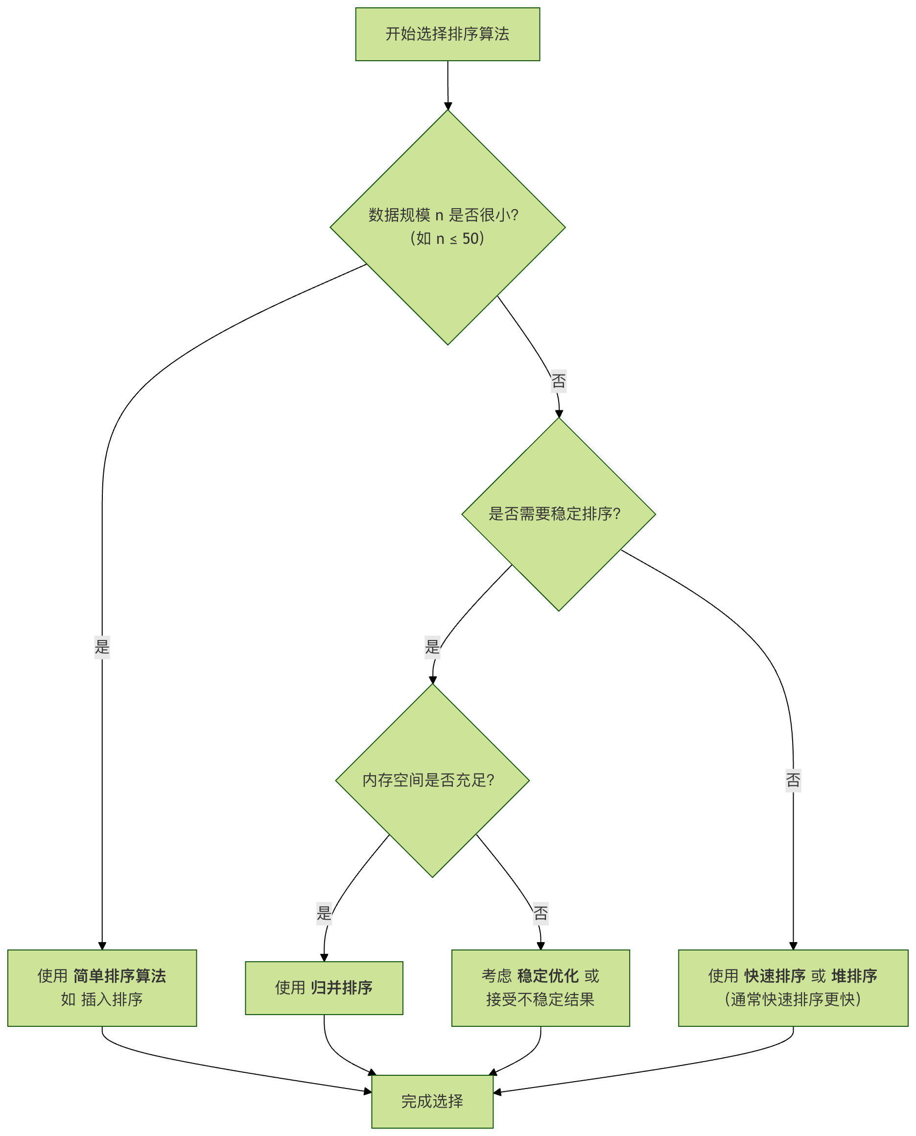
The following flowchart shows how to make a preliminary choice among several classic algorithms according to different requirement scenarios:
O(n²) level basic sorting algorithms
These algorithms are simple in concept and are the starting point for understanding sorting logic.
Bubble Sort
Core ideaRepeatedly "traverse" the sequence to be sorted, comparing two adjacent elements at a time, and swapping them if they are in the wrong order. Each traversal bubbles the largest (or smallest) element in the current unsorted portion to its correct position.
Algorithm steps:
- Compare adjacent elements. If the first is greater than the second (for ascending order), swap them.
- Do the same for every pair of adjacent elements, from the first pair at the beginning to the last pair at the end. After this step, the last element will be the largest number.
- Repeat the above steps for all elements except the last one (because each round determines a final element).
- Continue repeating the above steps for fewer and fewer elements each time, until there is no pair of numbers to compare.
Code implementation:
Example
"""
Bubble Sort (Ascending)
:param arr: The list to be sorted
"""
n = len(arr)
# The outer loop controls the number of passes needed (n-1 passes)
for i in range(n - 1):
# The inner loop performs comparison and swapping of adjacent elements
# After each pass, the last i+1 elements are already sorted, so the comparison range is 0 to n-1-i
for j in range(0, n - 1 - i):
if arr[j] > arr[j + 1]: # If the previous element is larger than the following element
# Swap the positions of the two elements
arr[j], arr[j + 1] = arr[j + 1], arr[j]
return arr
# Test data
test_data = [64, 34, 25, 12, 22, 11, 90]
print("Original array:", test_data)
sorted_data = bubble_sort(test_data.copy()) # Use a copy to avoid modifying the original data
print("After bubble sort:", sorted_data)
Output:
原始数组: [64, 34, 25, 12, 22, 11, 90]
冒泡排序后: [11, 12, 22, 25, 34, 64, 90]
Performance analysis:
- Time complexityBest case O(n) (achievable with optimization when already sorted), worst and average cases O(n²).
- Space complexity: O(1), it is an in-place sort.
- Stability: stable.
Selection Sort
Core ideaFind the smallest (or largest) element in the unsorted sequence, place it at the beginning of the sorted sequence, then continue to find the smallest (largest) element from the remaining unsorted elements and place it at the end of the sorted sequence. Continue in this way until all elements are sorted.
Algorithm steps:
- Initial state: the entire sequence is the unsorted region.
- In the i-th round (i starting from 0) of sorting, the current unsorted region is
arr[i...n-1]From this region, select the record with the smallest keyarr[min_index]。 - will
arr[min_index]With the first record of the unsorted regionarr[i]Swap. In this way,arr[0...i]Then the sorted region is formed. - After n-1 rounds, the array is sorted.
Code implementation:
Example
"""
Selection Sort (Ascending)
:param arr: The list to be sorted
"""
n = len(arr)
for i in range(n):
# Assume the element at the current index i is the smallest
min_index = i
# Find a smaller element in the range from i+1 to n-1
for j in range(i + 1, n):
if arr[j] < arr[min_index]:
min_index = j # Update the index of the smallest element
# Swap the found smallest element with the element at position i
arr[i], arr[min_index] = arr[min_index], arr[i]
return arr
# Test
test_data = [64, 25, 12, 22, 11]
print("Original array:", test_data)
print("After selection sort:", selection_sort(test_data.copy()))
Output:
原始数组: [64, 25, 12, 22, 11]
选择排序后: [11, 12, 22, 25, 64]
Performance analysis:
- Time complexityAlways O(n²), because complete comparisons are required regardless of whether the data is sorted.
- Space complexity: O(1), in-place sort.
- Stability:unstable. For example, the sequence
[5, 8, 5, 2, 9], in the first round, the first [element] will be5and2swapped, breaking the two5The original order.
Insertion Sort
Core ideaBy building an ordered sequence, for unsorted data scan backward through the sorted sequence, find the appropriate position, and insert it. This is like arranging playing cards.
Algorithm steps:
- Treat the first element as the sorted sequence.
- Take the next element and scan backward through the sorted element sequence.
- If the sorted element is greater than the new element, move the sorted element to the next position.
- Repeat step 3 until you find a position where the sorted element is less than or equal to the new element.
- After inserting the new element into this position.
- Repeat steps 2-5 until all elements are processed.
Code implementation:
Example
"""
Insertion Sort (Ascending)
:param arr: The list to be sorted
"""
n = len(arr)
# Start from the second element (index 1) because the first element is already sorted by default
for i in range(1, n):
key = arr[i] # The current element to be inserted
j = i - 1 # Index of the last element in the sorted sequence
# Scan the sorted sequence from back to front to find the insertion position of key
# At the same time, move elements greater than key one position backward
while j >= 0 and key < arr[j]:
arr[j + 1] = arr[j]
j -= 1
# Insert key into the correct position found
arr[j + 1] = key
return arr
# Test
test_data = [12, 11, 13, 5, 6]
print("Original array:", test_data)
print("After insertion sort:", insertion_sort(test_data.copy()))
Output:
原始数组: [12, 11, 13, 5, 6]
插入排序后: [5, 6, 11, 12, 13]
Performance analysis:
- Time complexityBest case O(n) (already sorted), worst and average cases O(n²).
- Space complexity: O(1), in-place sort.
- Stability: stable.
- Features: For small-scale or nearly sorted data, insertion sort is very efficient. It is the algorithm that advanced sorting algorithms (such as Timsort) switch to for small-scale data.
O(n log n) level efficient sorting algorithms
When the data size grows, O(n²) algorithms become very slow. The following more efficient algorithms are the mainstay of engineering practice.
Quicksort
Core idea:Divide and conquerSelect a pivot element. Through one pass of sorting, partition the records to be sorted into two independent parts, where the keys of one part are all smaller than the keys of the other part; then sort these two parts separately to make the whole sequence ordered.
Algorithm steps:
- Select pivotPick an element from the sequence and call it the "pivot".
- Partition OperationRearrange the sequence so that all elements smaller than the pivot are placed before it and all elements greater than the pivot are placed after it (equal numbers can go on either side). After this partition exits, the pivot is in its final position in the middle of the sequence. This is called the partition operation.
- recursively sortRecursively sort the sub-sequence with elements smaller than the pivot and the sub-sequence with elements greater than the pivot.
Code implementation:
Example
"""
Quick Sort (Ascending) - Main Function
"""
def _quick_sort(arr, low, high):
if low < high:
# pi is the partition index, arr[pi] is now in the correct position
pi = partition(arr, low, high)
# Recursively sort the subarrays before and after the partition
_quick_sort(arr, low, pi - 1)
_quick_sort(arr, pi + 1, high)
def partition(arr, low, high):
"""
Partition function, select the last element as the pivot
:return: the final correct position index of the pivot element
"""
pivot = arr[high] # Choose a pivot
i = low - 1 # Points to the end of the subarray of elements less than the pivot
for j in range(low, high):
# If the current element is less than or equal to the pivot
if arr[j] <= pivot:
i += 1
arr[i], arr[j] = arr[j], arr[i] # Swap
# Place the pivot element in the correct position (i+1)
arr[i + 1], arr[high] = arr[high], arr[i + 1]
return i + 1
_quick_sort(arr, 0, len(arr) - 1)
return arr
# Test
test_data = [10, 80, 30, 90, 40, 50, 70]
print("Original array:", test_data)
print("After quick sort:", quick_sort(test_data.copy()))
Output:
原始数组: [10, 80, 30, 90, 40, 50, 70]
快速排序后: [10, 30, 40, 50, 70, 80, 90]
Performance analysis:
- Time complexityAverage case O(n log n), worst case O(n²) (when the array is already sorted or reverse sorted and the pivot is chosen poorly). The worst case can be largely avoided by randomly selecting the pivot or using the "median-of-three" method.
- Space complexity: Average O(log n) (recursive call stack), worst-case O(n).
- Stability:unstable。
Merge Sort
Core idea:Divide and conquerA typical application. Merge already ordered subsequences to obtain a completely ordered sequence. That is, first make each subsequence ordered, and then make the subsequence segments ordered relative to each other.
Algorithm steps:
- DivideDivide the current interval into two parts, i.e., find the split point
mid = (low + high)/2。 - ConquerRecursively [sort] the two subintervals
arr[low...mid]andarr[mid+1...high]Perform merge sort. The termination condition for recursion is that the sub-interval length is 1 (one element is considered naturally ordered). - MergeMerge two sorted sub-intervals into one ordered interval.
Code implementation:
Example
"""
Merge Sort (Ascending) - Main Function
"""
if len(arr) > 1:
mid = len(arr) // 2 # Find the midpoint and split the array
left_half = arr[:mid]
right_half = arr[mid:]
# Recursively sort the left and right halves
merge_sort(left_half)
merge_sort(right_half)
# Merge the two sorted subarrays
i = j = k = 0
# Compare elements of the left and right subarrays, put the smaller one into the original array
while i < len(left_half) and j < len(right_half):
if left_half[i] < right_half[j]:
arr[k] = left_half[i]
i += 1
else:
arr[k] = right_half[j]
j += 1
k += 1
# Check if there are any remaining elements (left half or right half)
while i < len(left_half):
arr[k] = left_half[i]
i += 1
k += 1
while j < len(right_half):
arr[k] = right_half[j]
j += 1
k += 1
return arr
# Test
test_data = [38, 27, 43, 3, 9, 82, 10]
print("Original array:", test_data)
print("After merge sort:", merge_sort(test_data.copy()))
Output:
原始数组: [38, 27, 43, 3, 9, 82, 10]
归并排序后: [3, 9, 10, 27, 38, 43, 82]
Performance analysis:
- Time complexityBest, worst, and average cases are all O(n log n). Performance is very stable.
- Space complexityO(n), requiring extra space equal to the original array for merging.
- Stability: stable.
Heap Sort
Core idea: usingHeapA sorting algorithm designed for this data structure. A heap is an approximately complete binary tree structure that also satisfies the heap property: the value of a parent node is always greater than or equal to (max-heap) or less than or equal to (min-heap) any child node's value.
Algorithm steps:
- Build max heapConstruct the sequence to be sorted into a max-heap. At this point, the maximum value of the entire sequence is the root node at the top of the heap.
- Swap the top of the heap with the last elementSwap the top element (the maximum) with the last element; the last element is now the maximum.
- Adjust heap structure: for the remaining
n-1Reconstruct the remaining elements into a max-heap, which yields the next largest value. Swap it with the new last element (position n-1). - Repeat executionRepeat steps 2 and 3 until the heap size is 1; sorting is complete.
Code implementation:
Example
"""
Heap Sort (Ascending) - Using Max Heap
"""
n = len(arr)
# Step 1: Build the max heap. Start adjusting upward from the last non-leaf node
# Index of the last non-leaf node = n//2 - 1
for i in range(n // 2 - 1, -1, -1):
heapify(arr, n, i)
# Steps 2 & 3: Extract the top element (maximum) one by one and adjust the heap
for i in range(n - 1, 0, -1):
# Swap the current top element (maximum) with the last element
arr[i], arr[0] = arr[0], arr[i]
# Adjust the remaining elements to make it a max heap again, with heap size set to i
heapify(arr, i, 0)
return arr
def heapify(arr, n, i):
"""
Adjust the subtree rooted at i to make it a max heap
:param arr: heap array
:param n: current heap size
:param i: index of the current root
"""
largest = i # Initialize the maximum value as the root
left = 2 * i + 1 # Left child index
right = 2 * i + 2 # Right child index
# If the left child exists and is greater than the root
if left < n and arr[left] > arr[largest]:
largest = left
# If the right child exists and is greater than the current maximum
if right < n and arr[right] > arr[largest]:
largest = right
# If the maximum is not the root, swap and recursively adjust the broken sub-heap
if largest != i:
arr[i], arr[largest] = arr[largest], arr[i]
heapify(arr, n, largest)
# Test
test_data = [4, 10, 3, 5, 1]
print("Original array:", test_data)
print("After heap sort:", heap_sort(test_data.copy()))
Output:
原始数组: [4, 10, 3, 5, 1]
堆排序后: [1, 3, 4, 5, 10]
Performance analysis:
- Time complexityBest, worst, and average cases are all O(n log n).
- Space complexity: O(1), in-place sort.
- Stability:unstable。
Summary of algorithm performance comparison
To compare the characteristics of the above algorithms more intuitively, we summarize them in the following table:
| Algorithms | Average time complexity | Worst-case time complexity | Space complexity | Stability | Main Features |
|---|---|---|---|---|---|
| Bubble Sort | O(n²) | O(n²) | O(1) | Stable | Simple, low efficiency, suitable for teaching. |
| Selection Sort | O(n²) | O(n²) | O(1) | unstable | Fewer swaps, but a fixed large number of comparisons. |
| Insertion Sort | O(n²) | O(n²) | O(1) | Stable | Efficient for small-scale or nearly sorted data. |
| Quicksort | O(n log n) | O(n²) | O(log n) | unstable | Best average performance, is the most widely used sorting algorithm. |
| Merge Sort | O(n log n) | O(n log n) | O(n) | Stable | Stable performance, but requires extra space. Often used for external sorting. |
| Heap Sort | O(n log n) | O(n log n) | O(1) | unstable | In-place sorting and O(n log n) even in the worst case. |
Practice exercises
After theoretical learning, hands-on practice is the best way to consolidate knowledge.
Exercise 1: Algorithm selection and implementation
Given the following scenarios, which sorting algorithm would you choose? Briefly explain your reasons.
- Sort an array containing 10 numbers.
- Sort a linked list of 1 million student objects by student ID, requiring stability.
- Sort a large array in an embedded system with limited memory.
- Need to obtain the top K largest elements from a data stream in real time.
Reference answer approach:
- Insertion SortSmall data size; insertion sort is simple, friendly to nearly sorted data, and has a small constant factor.
- Merge SortLarge data size, stable sorting is required, and the linked list structure allows merge sort's merge operation to be completed in O(1) space (just by modifying pointers).
- Heap SortLimited memory, in-place sorting is needed, and heap sort guarantees O(n log n) performance even in the worst case.
- Maintain a min-heap of size KTraverse the data stream and use a heap to maintain the current K largest elements. This is not a complete sort, but it exploits the properties of a heap.
Exercise 2: Code debugging and optimization
The bubble sort below has a small bug and one place that can be optimized; please find and fix them.
Example
n = len(arr)
for i in range(n):
for j in range(n - 1):
if arr[j] > arr[j]:
arr[j], arr[j+1] = arr[j+1], arr[j]
return arr
Hint:
- Comparison Condition
arr[j] > arr[j]Always false. - The boundary of the inner loop can be optimized, because after each round, the trailing elements are already sorted.
Exercise 3: Hands-on implementation
Try to implement it yourself from scratchQuicksort, and think:
- If the benchmark
pivotWhat happens if the first element is always chosen as the pivot, when sorting an already sorted array? - How to modify
partitionModify the partition function so that it becomes a "three-way quicksort", which can handle arrays with many duplicate elements more efficiently.